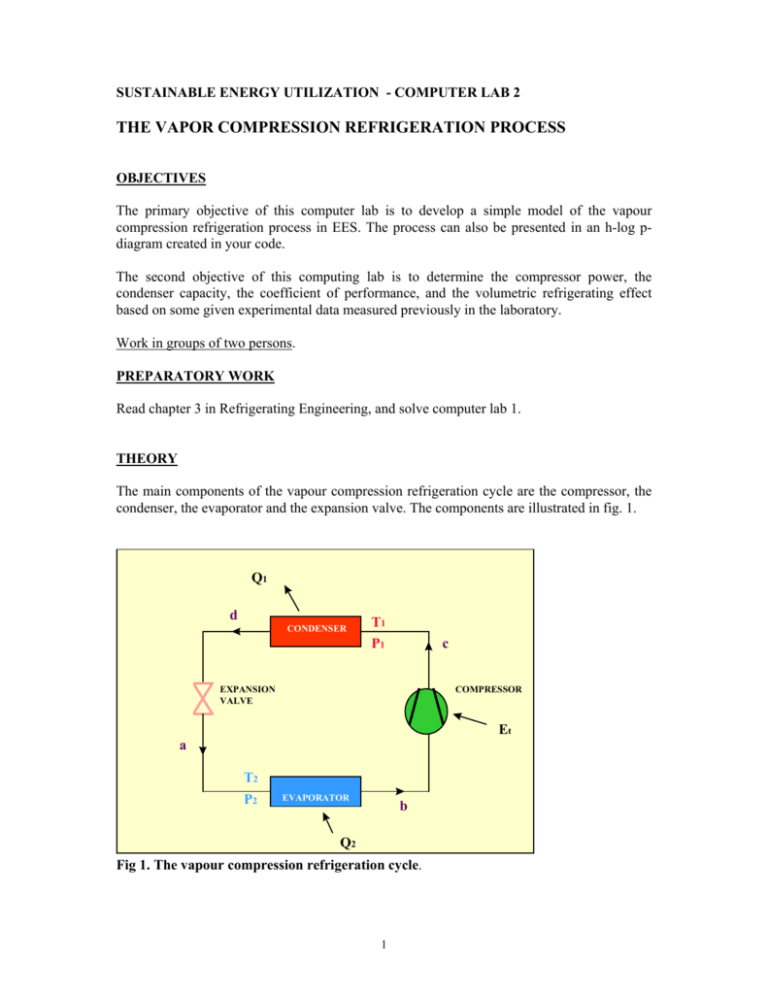
SUSTAINABLE ENERGY UTILIZATION - COMPUTER LAB 2
THE VAPOR COMPRESSION REFRIGERATION PROCESS
OBJECTIVES
The primary objective of this computer lab is to develop a simple model of the vapour
compression refrigeration process in EES. The process can also be presented in an h-log pdiagram created in your code.
The second objective of this computing lab is to determine the compressor power, the
condenser capacity, the coefficient of performance, and the volumetric refrigerating effect
based on some given experimental data measured previously in the laboratory.
Work in groups of two persons.
PREPARATORY WORK
Read chapter 3 in Refrigerating Engineering, and solve computer lab 1.
THEORY
The main components of the vapour compression refrigeration cycle are the compressor, the
condenser, the evaporator and the expansion valve. The components are illustrated in fig. 1.
Q1
d
CONDENSER
T1
P1
c
EXPANSION
VALVE
COMPRESSOR
Et
a
T2
P2
EVAPORATOR
b
Q2
Fig 1. The vapour compression refrigeration cycle.
1
The refrigerating capacity may be expressed as:
& =m
& r ⋅ (h 2k − h s )
Q
2
& r is the mass flow of the circulated refrigerant, h2k is the enthalpy after the
where m
evaporator and hs is the enthalpy before the evaporator
P [kPa]
R134a
10 4
(2,2)
(1,1)(5,5)
cis c
60 C
d
10 3
30 C
0.3 C
b
(3,3)
a
10 2
10 1
0
(4,4)
-25 C
50
100
150
200
250
h 2k
hs
300
h 1k,is h 1k
Fig 2. The vapour-compression refrigeration cycle represented in h – log P diagram.
The condenser heat capacity can be obtained from:
& =m
& r ⋅ ( h 1k − h s )
Q
1
where hs is the enthalpy after the condenser and h1k is the enthalpy before the condenser.
The compressor power may be expressed as:
E& t = m& r ⋅ (h1k − h2 k )
The power demand for an isentropic (ideal) compressor can be obtained from
2
350
h [kJ/kg]
& r ⋅ ( h 1k ,is − h 2 k )
E& is = m
where h1k,is is the isentropic enthalpy after the compressor The isentropic compressor
efficiency can be defined as
η is =
(h1k ,is − h2 k )
(h1k − h2 k )
The volumetric refrigerating effect, qv, is defined as
qv =
(h2k − hS )
v2k
where v2k is the specific volume at the compressor inlet.
In the computer lab file, lab2.ess, the real isentropic efficiency for a compressor tested in the
laboratory is calculated by the built-in formula. The data have been fitted to a function of the
two pressures, p1 and p2, according to fig 3.
0.90
0.80
0.70
η is
0.60
0.50
0.40
0.0 1.0 2.0 3.0 4.0 5.0 6.0 7.0 8.0 9.0 10.0 11.0 12.0
P1/P2
Fig 3. The isentropic efficiency for the tested compressor
This curve is unique for each compressor and different compressor types have different
characteristics.
The volumetric efficiency of the compressor can be calculated from
&
V
2
ηs = &
VS
3
& is the real volume flow at the compressor intake that can be calculated from the
where V
2
following equation
& =m
& r ⋅ v2k
V
2
& , can be obtained from the compressor geometry and given
The swept volume flow, V
S
characteristics as:
D2
n
&
VS = z ⋅ π ⋅ ( ) ⋅ S ⋅
4
60
(m3/s)
where
z : number of cylinders
D : cylinder diameter (m)
S : length of stroke (m)
n : number of revolutions (rpm)
The Pressure ratio, Pii, is defined as
Pii =
P1
P2
PROGRAM AND PRESENTATION IN DIAGRAMS
Write a program in EES that calculates the state points before and after each component in the
vapor compression refrigeration process in a h-log p-diagram for R134a (similar to figure 2),
the volumetric refrigerating effect, the condenser capacity, the volumetric efficiency of the
compressor and the COP2
1. The EES program Lab2 can be downloaded from the course homepage. Save the
program in your own catalogue.
2. Write the program in EES using the relevant equations from the theory and the
following instructions.
3. Select the high temperature, T1, equal to (35°C + average of your birth months); the
low temperature, T2, equal to -10°C, and the refrigeration capacity equal to 60 kW.
4. The compressor has the following dimensions:
z=2
D = 125 [mm]
S = 94 [mm]
n = 1450 rpm
4
5. Calculate the high pressure, the low pressure, the enthalpies after each component, and
Entropy and specific volume (Volume in EES Function Information command) before
the compressor. Select the Function Information command from the Options menu
and click on the Fluid properties button. The refrigerant is R134a.
Hint: Use the quality x in the function info to calculate some of the variables, e.g.,
calculate the pressures with temperature and quality, x, equal to 1 or 0.
6. Draw h-log P diagram for R134a. Select Property Plot from the Plot menu. Choose
R134a, P-h as plot type and OK.
7. To draw the refrigeration cycle on the P-h diagram, construct two vectors at the
Equation windows. One vector is needed for the pressures and the other for the
enthalpies. The vectors have indices one to five, equivalent with the five points (1,1),
(2,2), (3,3), (4,4), (5,5), in fig 2. The point (1,1) equals the point (5,5). EES array
variables have the array index in square brackets, e.g., X[5]. In most ways, array
variables are just like ordinary variables. (More information about Arrays is in the Help
menu).
Hint: you can construct your arrays by selecting the Insert/Modify Array from the
Edit menu. Enter a name for your array and then insert your variables. Rows
correspond to the numbers of points on the plot and in the column you set the
coordinate. You will have to construct two arrays – one for the pressure and the
other for the enthalpy variables in order to give two coordinates for each point.
Solve the equation window. Select Solve from the Calculate menu.
8. Plot the vectors in the h-log p-diagram. Select Overlay plot from the Plot menu. Click
automatic update and OK.
& , Q
& , E& , q, the pressure
9. Construct a parametric table containing the variables, T2, Q
2
1
t
ratio Pii, the isentropic efficiency ηis, the volumetric efficiency ηs and COP2. Enter the
following experimental values obtained from a compressor test rig for the low
& , for which the other variables
temperature, T2 and for the refrigeration capacity, Q
2
are to be determined. The other variables are to be calculated by your program.
T2 [°C]
10
0
-10
-20
-30
& [kW]
Q
2
150
98
60
33
15
& , as a function of the temperature, T2, in Plot Windows 2.
10. Plot, Q
1
5
11. Plot, E& t , as a function of the temperature, T2, in Plot Windows 3.
12. Plot, COP2, as a function of the temperature, T2, in Plot Window 4.
13. Plot, qv, as a function of the temperature, T2, in Plot Window 5.
14. Plot the isentropic efficiency ηis, as a function of the pressure ratio, Pii, in Plot Window 6.
15. Plot the volumetric efficiency, ηs, as a function of the pressure ratio, Pii, in Plot Window 7.
CONCLUSIONS
Hint: In order to answer some of the questions it will be helpful to build another plot
& r and v2k vs T2.
for m
1. Why does the compressor power, E& t , increase when the low temperature, T2, rise?
Are the results reasonable?
& , for the
2. How does the low temperature, T2, influence the condenser capacity, Q
1
vapour compression system?
3. How does the low temperature, T2, influence the coefficient of performance,
COP2, for the vapour compression system ?
4. Are the results of the volumetric refrigerating effect, qv, logical?
5. How does the pressure ratio, Pii, influence the isentropic efficiency, ηis? Why?
6. How does the pressure ratio, Pii, influence the volumetric efficiency, ηs? Why?
Write a short report that includes your answers to these questions and attach the
corresponding plots in a word (or pdf) file. Submit the file through Bilda, the file name
should be:
Lab2_Surname1_given name1_Surname2_given name2.doc (or .pdf).
Surname1_given name1 is the name of the first group member, and
Surname2_given name2 is the name of the second group member
Each group member need to submit the report individually eventhough you work in a
group!
To receive bonus for the exam, deadline for submission is November 26, 2007.
6