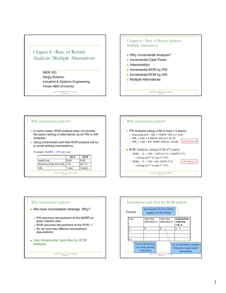
Chapter 8 – Rate of Return Analysis:
Multiple Alternatives
Chapter 8 - Rate of Return
„
Analysis: Multiple Alternatives
„
„
„
INEN 303
Sergiy Butenko
Industrial & Systems Engineering
Texas A&M University
Chapter 8 Rate of Return Analysis: Multiple
Alternatives
„
„
„
„
$100
‰
‰
– RORA: 0 = -100 + 16(P/A,i*,5) +100(P/F,i*,5)
– solving for i* we get i*=16%
– RORB: 0 = -100 + 201.14(P/F,i*,5)
will choose A
– solving for i* we get i*=15%
Alt B
$100
201.14
Life
5 years
Chapter 8 Rate of Return Analysis: Multiple
Alternatives
‰
‰
4
Incremental cash flow for ROR analysis
We have inconsistent rankings. Why?
‰
Chapter 8 Rate of Return Analysis: Multiple
Alternatives
3
Why incremental analysis?
„
One cycle of A: -100 + 116(P/F,10%,1) = 5.45
PWA = 5.45 + 5.45(P/A,10%,4) = 22.74
will choose B
PWB = -100 + 201.14(P/F,10%,5) = 24.89
■ ROR Analysis: (using LCM of 5 years)
Revenue at the end of life 116
1 year
PW Analysis (using LCM of lives = 5 years):
‰
Example: MARR = 10% per year
Initial Cost
2
Why incremental analysis?
In some cases, ROR analysis does not provide
the same ranking of alternatives as do PW or AW
analyses.
Using incremental cash flow ROR analysis will try
to avoid ranking inconsistency.
Alt A
Chapter 8 Rate of Return Analysis: Multiple
Alternatives
1
Why incremental analysis?
„
Why Incremental Analysis?
Incremental Cash Flows
Interpretation
Incremental ROR by PW
Incremental ROR by AW
Multiple Alternatives
Format:
PW assumes reinvestment at the MARR (or
given interest rate)
ROR assumes reinvestment at the ROR, i*
So we have two different reinvestment
assumptions
Incremental CF at 0 will be
negative in this format
Year
Cash flow
Alternative A
Cash flow
Alternative B
Incremental
cash flow
= B- A
0
$
$
$
1
…
„
n
Use incremental cash flow for ROR
analysis.
Chapter 8 Rate of Return Analysis: Multiple
Alternatives
Use LCM of lives
(or) study period,
if specified
5
As a convention, assume
B has the larger initial
investment
Chapter 8 Rate of Return Analysis: Multiple
Alternatives
6
1
Incremental cash flow for ROR analysis
„
Incremental cash flow for ROR analysis
Example 8.1:
Machine A
Initial cost - $15,000
Operating cost - $8200/yr
5% salvage value
25-year life
Machine B
Initial cost - $21,000
Operating cost - $7000/yr
5% salvage value
25-year life
„
Example 8.1, Solution:
Cash Flow
Year
0
1-25
25
Total
Machine A
-15,000
-8,200
750
-219,250
Inc. Cash Flow
Machine B
-21,000
-7,000
1,050
-194,950
B-A
-6,000
1,200
300
24,300
Create the Incremental Cash Flow Table.
Chapter 8 Rate of Return Analysis: Multiple
Alternatives
7
Chapter 8 Rate of Return Analysis: Multiple
Alternatives
9
Chapter 8 Rate of Return Analysis:
Multiple Alternatives
8
Incremental cash flow for ROR analysis
„
Example 8.2:
Type A
Type B
Initial cost - $70,000
AOC - $9000
Salvage Value - $5000
8-year life
Initial cost - $95,000
AOC - $7000
Salvage Value - $10,000
12-year life
Create the Incremental Cash Flow Table.
Chapter 8 Rate of Return Analysis: Multiple
Alternatives
Interpretation
10
Interpretation
The question is:
Is it worth spending additional $(B-A) to move from
investment A to investment B?
Example 8.3 (MARR = 10%):
Year
Compute ROR of the incremental investment, ∆i*B-A, to see…
If the ROR of the incremental cash flow equals
or exceeds the MARR, the alternative
associated with the extra investment should be
selected.
B
B- A
0
$-30,000
-50,000
$-20,000
1
-15,000
10,000
25,000
2
20,000
30,000
10,000
3
40,000
25,000
-15,000
4
5,000
-2,000
PWA = $6,360,22
PWB = $1,301.14
A
RORA = 16.36%
RORB = 11.33%
-7,000
So both feasible to
be considered.
RORB-A is infeasible (not positive) (see Excel file ch8)
Conclusion: the incremental investment is not justified: select A
Chapter 8 Rate of Return Analysis: Multiple
Alternatives
11
Chapter 8 Rate of Return Analysis: Multiple
Alternatives
12
2
Incremental ROR by PW Equation
Incremental ROR by PW
Mutually Exclusive Alternatives:
„
Required elements
‰
1.
INDEPENDENT - Selection of one alternative
does not effect the selection of others.
2.
‰
MUTUALLY EXCLUSIVE - Selection of one
alternative precludes the selection of
others.
‰
No incremental investment comparison
needed. Select all projects with ROR ≥
MARR.
Chapter 8 Rate of Return Analysis: Multiple
Alternatives
13
Incremental ROR by PW
„
Procedure
1. Order the alternatives by initial investment cost with the larger one
being alternative B.
2. Develop the cash flow and incremental cash flow series over the
LCM of lives.
3. Draw an incremental cash flow diagram, if needed.
4. Count the number of sign changes in the incremental cash flow
series to determine if multiple ROR may be present. If necessary,
use Norstrom’s criterion on the cumulative incremental cash flow
series to determine if a single positive root exists.
5. Set up the PW equation for the incremental cash flows and
determine ∆i*B-A.
6. Select the economically better alternative as follows:
If ∆i*B-A < MARR, select alternative A.
If ∆i*B-A > MARR, the extra investment is justified; select
alternative B.
Chapter 8 Rate of Return Analysis: Multiple
Alternatives
Example 8.4, Solution: (also see p284-286)
Incremental Cash Flow Table:
Year CF A
CF B
Inc. CF
0
-8000
-13,000
-5000
1
-3500
-1600
1900
2
-3500
-1600
1900
3
-3500
-1600
1900
4
-3500
-1600
1900
5
-3500
-1600
1900
5
2000
-13,000
-11,000
6
-3500
-1600
1900
7
-3500
-1600
1900
8
-3500
-1600
1900
9
-3500
-1600
1900
10 -3500
-1600
1900
10 2000
2000
Total -43,000
-38,000
5000
It is generally advisable to use PW or AW at
MARR when multiple rates are indicated.
If ∆i*B-A < MARR then select A, else select B.
Independent Projects:
„
‰
Chapter 8 Rate of Return Analysis: Multiple
Alternatives
Incremental cash flow series
LCM of lives
14
Example 8.4: Given the following information on
Verizon’s choices for an equipment vendor,
determine which vendor should be selected if MARR
is 15% per year (Excel file ch8).
Initial Cost, $
Annual Costs, $
Salvage Value, $
Life, years
Vendor A
-8,000
-3,500
0
10
Vendor B
-13,000
-1,600
2,000
5
Chapter 8 Rate of Return Analysis: Multiple
Alternatives
15
16
„
Chapter 8 Rate of Return Analysis: Multiple
Alternatives
„
Cum. Inc. CF
-5000
-3100
-1200
700
2600
4500
Example 8.4, Solution (continue):
Number of roots analysis:
Descarte’s rule:
Number of sign changes: 3 Î At most 3 roots
-6500
-4600
-2700
-800
1100
3000
5000
10000
Norstrom’s rule: Number of sign changes of
cumulative incremental cash flow: 3 Î so not
applicable.
17
Chapter 8 Rate of Return Analysis: Multiple
Alternatives
18
3
Example 8.4, Solution (continued):
Use the ROR equation based on PW of the incremental cash flow.
0 = -5000 + 1900(P/A, ∆i,10) – 11,000(P/F, ∆i,5) + 2000(P/F, ∆i,10)
Example 8.4, Solution (continue):
Breakeven ROR Interpretation
Assume the reinvestment rate is equal to the resulting ∆i*B-A.
Solve for ∆i using trial/error, etc.
∆i = 12.65%
Note: In theory, there are three roots to the equation, however, there
is only one (12.65%) falling in the practically reasonable range. For
example, the other one is –216%, falling out of the range of
acceptable range of i* ( [-100%, +infinity)).
This analysis assumes that PWB-A(i) > 0 for i < ∆i*B-A and
PWB-A(i) < 0 for i > ∆i*B-A so that ROR analysis is
consistent with PW analysis at MARR
Since the ROR of 12.65% on the extra investment is less than the
15% MARR, the lower-cost vendor A is selected.
Chapter 8 Rate of Return Analysis: Multiple
Alternatives
Chapter 8 Rate of Return Analysis: Multiple
Alternatives
19
Incremental ROR by PW
20
Incremental ROR by PW
The ∆i* can be interpreted as the breakeven rate of
return value.
Example 8.5
Select A for
MARR in this
range
Select B for
MARR in this
range
For MARR<12.65%, vendor B is justified.
For MARR>12.65%, vendor A is selected.
If MARR=12.65%, the alternatives are equally
attractive.
IBM is considering buying a chip placement
machine. The machine cost 260K with annual
operating expense 25K and a salvage value of
25K after 10 years. A slightly used machine is
available for 150K with annual operating expense
of 40K and a salvage value of 20K after 10 years.
Which machine should be selected if MARR is
10% per year.
PW for
incremental
cash
flows, $
0
∆i* %
Breakeven ∆i*
Chapter 8 Rate of Return Analysis: Multiple
Alternatives
21
Incremental ROR by PW
Chapter 8 Rate of Return Analysis: Multiple
Alternatives
22
Example 8.5, Solution (continue):
ROR ANALYSIS:
Example 8.5, Solution: PW Analysis
-110 + 15(P/A, i*, 10) + 5(P/F, i*, 10) = 0
year
Alt A
Alt B
B-A
0
1-10
10
-150K
-40K
20K
-260K
-25K
25K
-110K
15K
5K
By trial and error, i* = 6.60 < 10%
Additional investment is not justified
PW = -110 + 15 (P/A, 0.1,10) + 5 (P/F, 0.1, 10)
= -110 + 92.20 + 1.76 < 0
additional investment is not justified
Chapter 8 Rate of Return Analysis: Multiple
Alternatives
23
Chapter 8 Rate of Return Analysis: Multiple
Alternatives
24
4
ROR evaluation by AW
Incremental ROR by PW
Using the AW relation, there are two
equivalent ways for ROR analysis:
Use incremental cash flows over the LCM of
alternative lives
0 = AW
1.
Conclusion:
B-A
If the ROR method is used to evaluate two or more
alternatives, use the incremental cash flow and ∆i* to
make the decision between alternatives.
OR
2.
Use actual cash flows for one life cycle,
0 = AWB -AWA
Chapter 8 Rate of Return Analysis: Multiple
Alternatives
Example 8.6: Two machines are being considered
for purchase. If MARR is 10%, which machine
should be bought?
Determine ∆i*B-A·
Select the economically better alternative
as follows:
If ∆i*B-A < MARR, select alternative A.
If ∆i*B-A > MARR, the extra investment
is justified; select alternative B.
„
26
ROR evaluation by AW
ROR evaluation by AW
„
Chapter 8 Rate of Return Analysis: Multiple
Alternatives
25
Machine B
$200
$700
Annual benefit
95
120
Salvage value
50
150
6
12
Useful life, in years
Note: The same assumptions still exist.
Chapter 8 Rate of Return Analysis: Multiple
Alternatives
Machine A
Initial cost
Chapter 8 Rate of Return Analysis: Multiple
Alternatives
27
28
a) Use incremental cash flows with LCM of lives=12 years
Year
A
B
B-A
0
-200
-700
-500
1
95
120
25
2
95
120
25
3
95
120
25
4
95
120
25
5
95
120
25
6
-55
120
175
7
95
120
25
8
95
120
25
9
95
120
25
10
95
120
11
95
120
25
25
12
145
270
125
ROR
43.26%
14.32%
1.32%
b) Use actual cash flows for one life cycle.
0 = AWB-A
= -500(A/P,∆i*,12)+25+
+ 150(P/F,∆i*,6)(A/P,∆i*,12) +
+ 100(A/F,∆i*,12)
Solve for ∆i*, ∆i*=1.32%
Select Machine A
AWA = -200(A/P,i*,6) + 95 + 50(A/F,i*,6)
AWB = -700(A/P,i*,12) + 120 + 150(A/F,i*,12)
Set
0 = AWB -AWA
And solve for i*, i*=1.32%
-55= (95+50-200), since it is
beginning of second cycle
Select Machine A
Salvage value added
Chapter 8 Rate of Return Analysis: Multiple
Alternatives
29
Chapter 8 Rate of Return Analysis: Multiple
Alternatives
30
5
ROR evaluation by AW
ROR evaluation by AW
Example 8.7: Given the following information on
Verizon’s choices for an equipment vendor,
determine which vendor should be selected if MARR
is 15% per year.
„
Vendor A
-8,000
-3,500
0
10
Initial Cost, $
Annual Costs, $
Salvage Value, $
Life, years
Vendor B
-13,000
-1,600
2,000
5
Chapter 8 Rate of Return Analysis: Multiple
Alternatives
„
Example 8.7, Solution:
AWA = -8,000(A/P,i,10) – 3,500
AWB = -13,000(A/P,i,5) + 2,000(A/F,i,5) – 1,600
AWB - AWA = 0
-13,000(A/P,i,5) + 2,000(A/F,i,5) + 8,000(A/P,i,10) +1,900 = 0
Using trial and error, i* = 12.65% < MARR
ÎSelect vendor A.
Chapter 8 Rate of Return Analysis: Multiple
Alternatives
31
Multiple Alternatives (more than two)
„
„
32
Multiple Alternatives
For example, suppose there are six alternatives to evaluate:
Alternative: A
B
C
D
E
F
i*B
i*C
i*D
i*E
i*F
ROR:
i*A
Compute i* for each alternative
individually and discard those with i* <
MARR.
Do incremental pairwise comparison for
the accepted alternatives in order of
smallest-to-largest initial investment.
Suppose only i*A, i*C, i*D, i*F >= MARR, so discard B and E.
Sort by decreasing initial investment, suppose the result is:
A
D
F(largest cost)
C(smallest cost)
better
better
Best of four alternatives
Chapter 8 Rate of Return Analysis: Multiple
Alternatives
33
Example 8.8: Four Alternative Building Locations
B
-275,000
35,000
30
34
Multiple Alternatives
Multiple Alternatives
A
Initial Cost, $ -200,000
Annual CF, $ 22,000
Life, years
30
Chapter 8 Rate of Return Analysis: Multiple
Alternatives
C
-190,000
19,500
30
D
_
-350,000
42,000
30
Example 8.8, Solution:
1. The alternatives are ordered by increasing initial cost.
2. Compare C with DN (Do-Nothing).
0 = -190,000 + 19,500(P/A, ∆i*,30)
∆i*= 9.61% < MARR; Location C eliminated.
MARR = 10%
Now, compare A with DN.
∆i*= 10.44% > MARR; DN eliminated.
Location A-defender; Location B-challenger
Use incremental ROR AW analysis to select the best location.
Chapter 8 Rate of Return Analysis: Multiple
Alternatives
35
Chapter 8 Rate of Return Analysis: Multiple
Alternatives
36
6
Example 8.8, Solution (cont.):
3. Compare B with A.
0 = -275,000 – (-200,000) + (35,000-22,000)(P/A, ∆i*,30)
Î (P/A, ∆i*, 30) = 5.7692
Î ∆i*=17.18%. > MARR,
so Alternative B is justified incrementally; A eliminated.
Chapter 8 Rate of Return Analysis: Multiple
Alternatives
37
Multiple Alternatives
B
-275,000
35,000
D _
-350,000
42,000
Compared
C to DN
A to DN
B to A
D to B
Incr. Cost, $
Incr. CF, $
-190,000
19,500
-200,000
22,000
-75,000
13,000
-75,000
7000
9.0909
10.44
5.7692
17.18
10.7143
8.53
Yes
No
B
B
Incr. Justified?
No
Yes
Alt. Selected
DN
A
Chapter 8 Rate of Return Analysis: Multiple
Alternatives
38
Example 8.9, Solution:
EXAMPLE 8.9 : A pipeline is to be laid, the cost for the
various size pipe are shown below. MARR is 8% and
the life of the pipeline is 15 years.
B
C
10,510 13,180
800
1,400
5,800 5,200
A
-200,000
22,000
(P/A,∆i*,30) 9.7436
∆i*, %
9.61
4. Compare D with B.
0 = -75,000 + 7000(P/A, ∆i*,30)
P/A value = 10.7143, ∆i*=8.53% < MARR
Location D eliminated; only Location B remains.
Location B is selected.
A
Initial Cost 9,180
Installation 600
Ann. Cost 6,000
C
Initial Cost, $ -190,000
CF, $
19,500
D
15,850
1,500
4,900
A vs. B (i.e B-A)
Initial Cost
- 11,310 + 9,780 = -1,530
Ann. Cost - 5,800 + 6,000 = 200
E
30,530
2,000
4,800
0 = 200(P/A, i*, 15) - 1530
(P/A, i*, 15) = 7.65
(P/A, .08, 15) = 8.56, therefore, i* > 8%
A is removed and B is the new defender
Chapter 8 Rate of Return Analysis: Multiple
Alternatives
39
Example 8.9, Solution (continue):
Chapter 8 Rate of Return Analysis: Multiple
Alternatives
40
Example 8.9, Solution (continue):
C vs. D
Initial Cost 14,580 - 17,350 = -2,770
Ann. Cost 5,200 - 4,900 = 300
B vs. C
Initial Cost 11,310 - 14,580 = -3270
Ann. Cost 5800 - 5200 = 600
0 = 300 (P|A, i*, 15) - 2770
(P/A, i*, 15) = 9.23 > 8.56 = (P/A, .08, 15)
0 = 600(P|A, i*, 15) - 3270
(P/A, i*, 15) = 5.45 < 8.56 = (P/A, .08, 15)
D is removed and C is the defender
B is removed and C is the new defender
Chapter 8 Rate of Return Analysis: Multiple
Alternatives
41
Chapter 8 Rate of Return Analysis: Multiple
Alternatives
42
7
Example 8.9, Solution (continue):
Example 8.9, Solution (continue):
PW(A) = -9,780 - (P/A, .08, 15) 6,000 = -61,137
C vs. E
Initial Cost 14,580 - 32,530 = -17,950
Ann. Cost 5200 - 4800 = 400
PW(B) = -11,310 - (P/A, .08, 15) 5,800 = -60,955
PW(C) = -14,580 - (P/A, .08, 15) 5,200 = -59,089
0 = 400 (P|A, i*, 15) - 17,950
(P/A, i*, 15) = 44.87 > 8.56 = (P/A, .08, 15)
PW(D) = -17,350 - (P/A, .08, 15) 4,900 = -59,291
PW(E) = -32,530 - (P/A, .08, 15) 4,800 = -73,615
C is the successful final alternative
Choose Largest PW, Alternative C
Chapter 8 Rate of Return Analysis: Multiple
Alternatives
43
Chapter 8 Rate of Return Analysis: Multiple
Alternatives
44
8