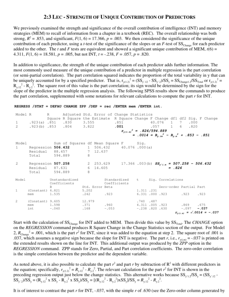
2:3 LEC - STRENGTH OF UNIQUE CONTRIBUTION OF PREDICTORS
We previously examined the strength and significance of the overall contribution of intelligence (INT) and memory
strategies (MEM) to recall of information from a chapter in a textbook (REC). The overall relationship was both
strong, R2 = .853, and significant, F(1, 6) = 17.366, p = .003. We then considered the significance of the unique
contribution of each predictor, using a t-test of the significance of the slopes or an F-test of SSChange for each predictor
added to the other. The t and F tests are equivalent and showed a significant unique contribution of MEM, t(6) =
4.311, F(1, 6) = 18.581, p = .005, but not INT, t = -.238, F = .057, p = .820.
In addition to significance, the strength of the unique contribution of each predictor adds further information. The
most commonly used measure of the unique contribution of a predictor in multiple regression is the part correlation
(or semi-partial correlation). The part correlation squared indicates the proportion of the total variability in y that can
be uniquely accounted for by a specified predictor. That is, ry(1.2)2 = (SSy’.12 - SSy’.2)/SSy = SSChange1.2/SSTotal or ry(1.2)2 =
Ry.122 - Ry.22. The square root of this value is the part correlation; its sign would be determined by the sign for the
slope of the predictor in the multiple regression analysis. The following SPSS results show the commands to produce
the part correlation, supplemented with some notations for relevant calculations to compute the part r for INT.
REGRESS /STAT = DEFAU CHANGE ZPP /DEP = rec /ENTER mem /ENTER int.
Model R
1
2
R
Square
.923(a) .851
.923(b) .853
Model
1
Regression
Residual
Total
2
Model
1
2
Adjusted
R Square
.830
.804
Std. Error of
the Estimate
3.555
3.822
Sum of Squares
506.432
88.457
594.889
Regression 507.258
Residual
87.631
Total
594.889
Change Statistics
R Square Change F Change
.851
40.076
.001
.057
ry(i.m)2 = .826/594.889
= .0014 = Ry.im2 -
df1 df2 Sig. F Change
1
7
.000
1
6
.820
Ry.m2
.853 - .851
df Mean Square F
Sig.
1 506.432
40.076 .000(a)
7 12.637
8
2
6
8
253.629
14.605
17.366 .003(b) SSy’i.m = 507.258 - 506.432
= .826
Unstandardized
Coefficients
B
(Constant) 6.821
mem
1.535
Standardized
Coefficients
Std. Error Beta
5.202
.242
.923
t
(Constant) 9.605
mem
1.598
int
-.040
12.979
.371
.168
.740 .487
4.311 .005 .923
-.238 .820 .630
.960
-.053
Sig. Correlations
Zero-order Partial Part
1.311 .231
6.331 .000 .923
.923
.923
.869
.675
-.097
-.037
ry(i.m) = .0014 = -.037
Start with the calculation of SSChange for INT added to MEM. Then divide this value by SSTotal. The CHANGE option
on the REGRESSION command produces R Square Change in the Change Statistics section of the output. For Model
2, RChange2 = .001, which is the part r2 for INT, since it was added to the equation at step 2. The square root of .001 is
.037, which assumes a negative sign because the slope for INT is negative. The part r, i.e., ry(i.m) = -.037 is printed on
the extended results shown on the line for INT. This additional output was produced by the ZPP option in the
REGRESSION command. ZPP stands for Zero, Partial, and Part correlation coefficients. The zero-order correlation
is the simple correlation between the predictor and the dependent variable.
As noted above, it is also possible to calculate the part r2 and part r by subtraction of R2 with different predictors in
the equation; specifically, ry(1.2)2 = Ry.122 - Ry.22. The relevant calculation for the part r2 for INT is shown in the
preceding regression output just below the change statistics. This alternative works because SSy’1.2/SSy = (SSy’.12 SSy’.2)/SSy = (Ry.122 x SSy - Ry.22 x SSy)/SSy = [(Ry.122 - Ry.22)xSSy]/SSy = Ry.122 - Ry.22.
It is of interest to contrast the part r for INT, -.037, with the simple r of .630 (see the Zero-order column generated by
the ZPP option). Note how a sizable positive correlation (.630) has become tiny and even slightly negative (-.037)
once its correlation with MEM is controlled. The original simple correlation was positive and large because people
high on intelligence (i.e., high on INT) tended to use good memory strategies (i.e., high on MEM), which was related
to performance (i.e., the criterion variable REC). Controlling for MEM eliminated the connection between INT and
REC. Work through the part correlation for MEM using the following analysis.
REGRESS /STAT = DEFAU CHANGE ZPP /DEP = rec /ENTER int /ENTER mem.
Model R
1
2
R
Square
.630(a) .397
.923(b) .853
Model
1
Regression
Residual
Total
2
Model
1
2
Adjusted
R Square
.310
.804
Std. Error of
the Estimate
7.162
3.822
Sum of Squares
235.878
359.011
594.889
Regression 507.258
Residual
87.631
Total
594.889
Change Statistics
R Square Change F Change df1 df2 Sig. F Change
.397
4.599
1
7
.069
.456
18.581
1
6
.005
df Mean Square F
1 235.878
4.599
7 51.287
8
2
6
8
253.629
14.605
Sig.
.069(a)
17.366 .003(b)
Unstandardized
Coefficients
B
(Constant) -9.772
int
.474
Standardized
Coefficients
Std. Error Beta
22.815
.221
.630
t
(Constant) 9.605
int
-.040
mem
1.598
12.979
.168
.371
.740 .487
-.238 .820 .630
4.311 .005 .923
-.053
.960
Sig. Correlations
Zero-order Partial Part
-.428 .681
2.145 .069 .630
.630
.630
-.097
.869
-.037
.675
Although the contribution of MEM remains significant and moderately strong even with INT in the equation, FChange
= 18.581, tm.i = 4.311, p = .005, rr(m.i)2 = .6752 = .456, note that the strength is considerably reduced with INT
controlled statistically (i.e., .675 is weaker than .923, the simple correlation between recall and memory strategy).
This is because some, but not all, of what MEM could predict when used alone was due to variability in MEM that
was shared with INT. Theoretically, INT MEM REC, but INT is not the only source of variability in MEM, so
that even when INT is controlled, there is still variation in MEM that is related to recall.
Note that the sum of the unique contributions of the two predictors does not add up to the total variability accounted
for when both predictors are in the equation; that is, rr(i.m)2 + rr(m.i)2 = -.0372 + .6752 = .457 < .853 = Rr.im2 (this
inequality could also be stated in terms of SSs). The other 40% or so of variability in REC that is predictable from
INT and MEM is due to variability shared by the two predictors (i.e., area c in the Venn diagrams).
Next class we examine a second correlation coefficient representing the unique contribution of a predictor, namely
the partial correlation coefficient. The partial correlation coefficient is used less frequently and must be interpreted
with much caution, as we will note. To set the stage for the partial correlation, note that SSChange could be calculated
by considering SSResidual in Models 1 and 2, rather than SSRegression. We have already noted that the increase in
SSRegression from Model 1 to Model 2 must be due to variability moving from SSResidual in Model 1, because SSTotal
remains exactly the same in both models. To illustrate for the unique contribution of INT, SSr’i.m = SSResidualModel1 SSResidualModel2 = 88.457 - 87.631 = .826, the same quantity calculated earlier. So SSChange equals not only the increase
in SSRegression when one predictor is added to the other, but also the decrease in SSResidual when one predictor is added to
the other. Appreciation of this point will help our understanding of partial correlation coefficients.
The previous material pointed out that SSChange for a predictor could be considered as either the increase in SSRegression
when a new predictor is added to the equation, or as a decrease in SSResidual when a new variable is added. The partial
correlation coefficient, ry1.2 (note absence of brackets), can best be conceptualized in terms of the latter view of
SSChange. In essence, ry1.22 reflects the proportion of residual variability from Model 1 that is now accounted for in
Model 2 with the added predictor. That is, ry1.22 = SSChange / SSResidualModel1 = SSChange / (SSTotal - SSy’.2).
Consider SSChange for INT, i.e., SSr’i.m = .826, which gave rr(i.m)2 = .826/594.889 = .0014 for the part correlation
squared, and rr(i.m) = .0014 = -.037. Instead of dividing by SSTotal, dividing by SSTotal - SSr’.m = 594.889 - 506.432 =
88.457, gives the partial r2 for INT, rr’i.m2 = .826 / 88.457 = .0093, and rr’i.m = .0093 = .0966. The partial r indicates
that intelligence accounts for .93% of the 88.457 units of variability in REC not already accounted for by MEM,
whereas the part (or semi-partial) r indicates that intelligence accounts for .14% of the total variability in recall.
The partial correlation appears in the ZPP portion of the regression output. The entry for INT, -.097, agrees with the
preceding calculations. The negative sign is added because of the negative sign of the slope for INT. The partial r
for MEM would be worked out in an analogous fashion.
Partial rs must be interpreted with caution. The partial r for INT is much larger than the part r (although still modest
because SSChange was so small), not because its contribution to prediction of recall was any stronger but because the
contribution of MEM alone was strong, thus removing much of the variability in y from the denominator, and
inflating the apparent strength of INT.
Although not a measure of strength in the same sense as correlation coefficients, information about the magnitude of
the change in y with changes in predictors can also be used to compare the contribution of different predictors. But
the unstandardized coefficients that we have considered so far are less than ideal for this purpose because the amount
of change in y depends not only on the relationship between y and the predictor, but also on the amount of variability
in the predictor. Specifically, a predictor with a large range of values could have a larger impact on y, even if its
slope was smaller, than a predictor with a small range of values, even if its slope was larger. For example, a predictor
with values ranging from 1 to 5 and a slope of 5.0 could produce predicted scores from 5 to 25, whereas a predictor
with values ranging from 5 to 100 and a smaller slope of 1.0 could produce predicted scores ranging from 5 to 100, a
much larger spread in y.
The solution to this problem is to calculate standardized regression coefficients, which will be based on predictor
and criterion variables all having the same amount of variability, in essence standardized variables with s = 1.0. The
problem with the unstandardized coefficients and the solution is illustrated below.
DESCR rec mem int.
rec
mem
int
N
9
9
9
Minimum
25
12
88
Maximum
51
27
118
Mean
38.89
20.89
102.67
Std. Deviation
8.623
5.183
11.456
COMPUTE zrec = (rec - 38.8889)/8.6233.
COMPUTE zmem = (mem - 20.8889)/5.1828.
COMPUTE zint = (int - 102.6667)/11.4564.
z = (y - M)/SD
DESCR zrec zmem zint.
zrec
zmem
zint
N
9
9
9
Minimum
-1.6106
-1.7151
-1.2802
Maximum
1.4045
1.1791
1.3384
Mean
-.000001
-.000002
-.000003
Std. Deviation
.9999987
All Ms = 0
.9999943
All SDs = 1
1.0000034
REGRESS /DEP = rec /ENTER mem int.
Model R
1
R Square Adjusted R
Square
.923(a) .853
.804
Model
1
Regression
Residual
Total
Model
1
Sum of Squares
507.258
87.631
594.889
Std. Error of
the Estimate
3.822
df Mean Square F
Sig.
2 253.629
17.366 .003(a)
6 14.605
8
Unstandardized
Coefficients
B
(Constant) 9.605
mem
1.598
int
-.040
Standardized
Coefficients
Std. Error Beta
12.979
.371
.960
.168
-.053
t
Sig.
.740 .487
4.311 .005
-.238 .820
REGRESS /DEP = zrec /ENTER zmem zint.
Model R
1
R Square Adjusted R
Square
.923(a) .853
.804
Model
1
Regression
Residual
Total
Model
1
Std. Error of
the Estimate
.4431800
Sum of Squares df Mean Square F
Sig.
6.822
2 3.411
17.366 .003(a)
1.178
6 .196
8.000
8
Unstandardized
Coefficients
B
(Constant) 6.16E-007
zmem
.960
zint
-.053
Standardized
Coefficients
Std. Error Beta
.148
.223
.960
.223
-.053
t
Sig.
.000 1.000
4.311 .005
-.238 .820
Standardized coefficients can be interpreted in terms of standard deviations. Specifically, the slope indicates the
amount of change in y in standard deviation units given a one standard deviation change in the predictor. Given a
one standard deviation change in INT, REC will decrease by .053 SDs. Given a one standard deviation change in
MEM, REC will increase by .960 SDs. Notice that these values, although still far apart, are closer to one another than
were the unstandardized coefficients, -.040 for INT and 1.598 for MEM. Adjusting for the differences in variability
of the predictors has changed somewhat their relative standing. In other cases, the change could be more marked; for
example, the predictor with the larger unstandardized coefficient could have the smaller standardized coefficient,
depending on the SDs for the respective predictors.
I will show some simulations in class to illustrate how the hypothesis testing procedures described for multiple
regression, whether the overall F or individual predictor ts or Fs, conform to our standard model. That is, when null
hypotheses are true, probability of rejecting is about .05 (or whatever alpha is), whereas when null hypotheses are
false, probability of rejecting is much greater than .05.
FURTHER ANALYSES OF NATIONAL TRUST EXAMPLE
Lecture 2:2 introduced a study of National Trust, with average Trust in 36 countries predicted by Individualism
(IDV) and Gross Domestic Product (GDP). Although both IDV and GDP contributed significantly to prediction of
Trust when entered alone in regression analyses, only GDP was a significant unique predictor of Trust in the multiple
regression analysis. The following analyses add measures of the strength of the unique contribution of each
predictor. Calculate the part and partial correlation coefficients for each predictor and show the correspondence with
values produced by SPSS using the CHANGE and ZPP options.
REGRESS /STAT = DEFAULT CHANGE ZPP /DEP = trust /ENTER gdp /ENTER idv.
Model R
1
2
R
Square
.557(a) .311
.590(b) .348
Adjusted
R Square
.290
.309
Std. Error of
the Estimate
12.9217107
12.7559837
Change Statistics
R Square Change F Change df1 df2 Sig. F Change
.311
15.326
1
34 .000
.037
1.889
1
33 .179
Model
Sum of Squares df Mean Square F
Sig.
1
Regression 2558.999
1 2558.999
15.326 .000(a)
Residual
5677.001
34 166.971
Total
2
2
35
Regression 2866.401
Residual
5369.599
2 1433.201
33 162.715
Total
35
Coefficients(a)
Model
1
8236.000
8236.000
Unstandardized
Coefficients
B
8.808
.001(b)
Standardized
Coefficients
Std. Error Beta
t
Sig. Correlations
(Constant) 26.232
gdp
.001
3.296
.000
.557
7.959 .000
3.915 .000 .557
.557
.557
(Constant) 19.510
gdp
.001
idv
.169
5.874
.000
.123
.418
.238
3.321 .002
2.415 .021 .557
1.374 .179 .483
.387
.233
.339
.193
Zero-order Partial Part
REGRESS /STAT = DEFAULT CHANGE ZPP /DEP = trust /ENTER idv /ENTER gdp.
Model R
1
2
R
Square
.483(a) .233
.590(b) .348
Adjusted
R Square
.210
.309
Std. Error of
the Estimate
13.6319656
12.7559837
Change Statistics
R Square Change F Change df1 df2 Sig. F Change
.233
10.320
1
34 .003
.115
5.830
1
33 .021
Model
Sum of Squares df Mean Square F
Sig.
1
Regression 1917.763
1 1917.763
10.320 .003(a)
Residual
6318.237
34 185.830
Total
2
8236.000
Regression 2866.401
Residual
5369.599
2 1433.201
33 162.715
Total
35
8236.000
Coefficients(a)
Model
1
2
35
8.808
.001(b)
Unstandardized
Coefficients
B
(Constant) 17.434
idv
.342
Standardized
Coefficients
Std. Error Beta
6.210
.107
.483
t
(Constant) 19.510
idv
.169
gdp
.001
5.874
.123
.000
3.321 .002
1.374 .179 .483
2.415 .021 .557
.238
.418
Sig. Correlations
Zero-order Partial Part
2.808 .008
3.212 .003 .483
.483
.483
.233
.387
.193
.339
One interesting feature of the preceding analyses is that the unstandardized regression coefficient for GDP (.001), the
predictor with the significant and stronger relationship with Trust, is much smaller than the coefficient for IDV
(.169), the predictor with a nonsignificant and weaker relationship with Trust. This occurs because of the marked
difference in s for the two predictors, as shown below. The /MISSING = LIST option instructs SPSS to ignore cases
with missing data on any variable for all of the variables, and is required because IDV has missing data. Without this
option, Trust and GDP statistics would be based on 42 countries and IDV statistics on 36 countries, making the SD
values not directly comparable. Note that the SD for GDP is almost 600 times larger than the SD for IDV. The
standardized regression analyses correct for this disparity in variability (see previous analyses) and represent the
relationships in terms of standard deviation units. The REGRESSION analysis below illustrates this.
DESCR trust, idv, gdp /MISSING = LIST.
N
36
36
36
trust
idv
gdp
Minimum
7.0000
18.0000
258.0000
Maximum
66.0000
91.0000
45951.0000
Mean
36.000000
54.222222
13984.777778
Std. Deviation
15.3399572
21.6189218
12242.3664872
COMPUTE ztrust = (trust -
36.000000)/15.3399572.
COMPUTE zidv
= (idv
-
54.222222)/21.6189218.
COMPUTE zgdp
= (gdp
- 13984.777778)/12242.3664872.
REGRE /DESCR /STAT = DEFAU ZPP /DEP = ztrust /ENTER zidv zgdp.
Descriptive Statistics
Mean
Std. Deviation
ztrust .000000 1.0000000
zidv
.000000 1.0000000
zgdp
.000000 1.0000000
N
36
36
36
Correlations
Pearson
ztrust
ztrust 1.000
zidv
.483
zgdp
.557
zidv
.483
1.000
.584
zgdp
.557
.584
1.000
Model R
1
R Square Adjusted R
Square
.590(a) .348
.309
Std. Error of
the Estimate
.8315528
Model
Sum of Squares df Mean Square F
Sig.
1
Regression 12.181
2 6.091
8.808 .001(a)
Residual
22.819
33 .691
Total
Model
1
35.000
Unstandardized
Coefficients
B
(Constant) .000
zidv
.238
zgdp
.418
35
Standardized
Coefficients
Std. Error Beta
.139
.173
.238
.173
.418
t
Sig.
Correlations
Zero-order Partial Part
.000 1.000
1.374 .179 .483
.233
.193
2.415 .021 .557
.387
.339
BIRTH RATE AND MORTALITY EXAMPLE
GET
FILE='F:\4\S\_Fall\REG\datasets\nations.sav'.
REGRESS /DESCR /STAT = DEFAU CHANGE ZPP
/DEP birth /ENTER chldmort /ENTER infmort
/SAVE PRED(prdb.ci) RES(resb.ci).
Crude birth
rate/1000
people
Child (1-4 yr)
mortality 1985
Infant (<1 yr)
mortality 1985
Mean Std. Deviation N
32.79 13.634
109
9.96
11.232
109
68.47 49.244
109
Pearson
Crude birth
Correlation rate/1000
people
Child (1-4 yr)
mortality 1985
Infant (<1 yr)
mortality 1985
Model R
1
2
Model
Crude birth
rate/1000
people
Child (1-4 yr)
mortality 1985
Infant (<1 yr)
mortality 1985
1.000
.777
.882
.777
1.000
.949
.882
.949
1.000
R
Adjusted Std. Error of Change Statistics
Square R Square the Estimate
R Square Change F Change df1 df2 Sig. F Change
.777(a) .604
.902(b) .813
.600
.810
8.618
5.947
Sum of Squares df
.604
.209
163.333
118.699
Mean Square F
Regression 12129.831
Residual
7946.316
Total
20076.147
1
12129.831
107 74.265
108
163.333 .000(a)
2
Regression 16327.536
Residual
3748.610
Total
20076.147
2
8163.768
106 35.364
108
230.848 .000(b)
1
(Constant)
Child (1-4 yr)
mortality 1985
2
(Constant)
Child (1-4 yr)
mortality 1985
Infant (<1 yr)
mortality 1985
107 .000
106 .000
Sig.
1
Model
1
1
Unstandardized
Coefficients
B
23.388
.944
Standardized
Coefficients
Std. Error Beta
1.106
.074
.777
t
12.536
-.728
1.255
.162
-.600
9.991 .000
-4.504 .000 .777
-.401
-.189
.402
.037
1.451
10.895 .000 .882
.727
.457
Residuals Statistics(a)
Minimum Maximum Mean Std. Deviation N
Predicted Value 14.95
52.36
32.79 12.296
109
Residual
-10.933 16.554 .000 5.891
109
Sig. Correlations
Zero-order Partial Part
21.153 .000
12.780 .000 .777
.777
.777
input program.
loop c = 0 to 50 by 10.
leave c.
loop i = 0 to 200 by 20.
end case.
end loop.
end loop.
end file.
end input program.
compute b = 12.536 - .728*c + .402*i.