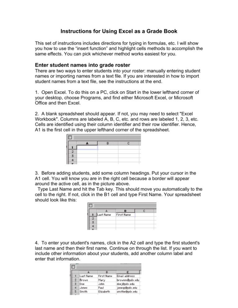
Instructions for Using Excel as a Grade Book
This set of instructions includes directions for typing in formulas, etc. I will show
you how to use the “insert function” and highlight cells methods to accomplish the
same effects. You can pick whichever method works easiest for you.
Enter student names into grade roster
There are two ways to enter students into your roster: manually entering student
names or importing names from a text file. If you are interested in how to import
student names from a text file, see the instructions at the end.
1. Open Excel. To do this on a PC, click on Start in the lower lefthand corner of
your desktop, choose Programs, and find either Microsoft Excel, or Microsoft
Office and then Excel.
2. A blank spreadsheet should appear. If not, you may need to select "Excel
Workbook". Columns are labeled A, B, C, etc. and rows are labeled 1, 2, 3, etc.
Cells are identified using their column identifier and their row identifier. Hence,
A1 is the first cell in the upper lefthand corner of the spreadsheet.
3. Before adding students, add some column headings. Put your cursor in the
A1 cell. You will know you are in the right cell because a border will appear
around the active cell, as in the picture above.
Type Last Name and hit the Tab key. This should move you automatically to the
cell to the right. If not, click in the B1 cell and type First Name. Your spreadsheet
should look like this:
4. To enter your student's names, click in the A2 cell and type the first student's
last name and then their first name. Continue on through the list. If you want to
include other information about your students, add another column label and
enter that information.
5. Once you have all of your students entered, save your file. Click on File in the
menu bar at the top of the page and select Save. I suggest you name your file in
such a way that it is clear as to which class and which semester it refers to. For
example, "PSY 113 F03 grades". Excel will add the necessary file extension
(".xls"). I have folders for each class so I save the gradebooks there, then they
are easy to find later on.
Label columns for assignments
Now that all of your students are entered, you will need to label the columns for
your graded assignments. Additional columns can be added at any time. For the
purpose of this exercise, we will add the following columns: Quiz 1, Quiz 2, Quiz
3, Mid-term, Final Exam, and Term Paper.
1. Put your cursor in cell D1 (or in row 1 of your first empty column) and type
Quiz 1.
2. Move to the next column (row 1) and type Quiz 2. If you hit the Tab key after
entering a label, your cursor will automatically be put in the next cell.
3. Complete the labeling of columns so that your spreadsheet now looks like that
below:
Enter grades
Now that the columns are labeled, you can begin entering grades. For the sake
of this exercise, we will fill in grades for all of your students and all of the
assignments. In a real course, you can enter grades at any time and edit them as
well.
1. To enter grades, put your cursor in the cell for a given student and a given
assignment.
2. Type in the grade. Hit the Enter key to move downward to the next student.
When done, your grade roster should like the one below:
If you want to calculate assignment means and standard
deviations -You can use Excel to calculate some simple statistics on your assignment
grades. These statistics can then be shared with your students. This is NOT a
necessary part of maintaining an excel gradebook, but might be interesting for
you and/or your students.
1. As usual, add some column labels first. Put your cursor in cell C7 and type
"Mean". Hit the enter key and type "Std deviation" in cell C8. Your spreadsheet
should look like the one below:
2. Now you need to type in cell D7 a formula for calculating the average (mean)
grade. Put your cursor in D7 and type (without the quotation marks)
"=average(D2:D5)" and hit the enter key. This formula tells Excel to calculate the
average grade for Quiz 1. Now put your cursor in D8 and we will type in the
formula to calculate the standard deviation. Type "=stdev(D2:D5)". Hit the enter
key. Your spreadsheet should look like this:
3. Then you can COPY the formulas created for Quiz 1 across for all of the
assignments. Put your cursor in D7 and drag down to D8 to highlight those two
cells.
4. Click on Edit in the menu at the top of the page and select "Copy". Click in E7
cell, hold down the cursor and drag it to I8, highlighting two rows beneath the
remainder of assignments. Let go of the cursor.
5. Click on Edit and then select "Paste". Means and standard deviations for all of
you assignments should appear:
Calculating total points for each student:
Once you have all your grades entered, you may use Excel to add up each of the
student's total points. This score can then be used to calculate a final letter grade
if you want. For this exercise, we will assume that the total possible points for all
of the assignments adds up to 345 pts and that there is no weighting of
assignments.
1. In the column to the right of Term Paper, add the column label Total Points.
Hit the enter key so that you are in the cell directly below the column label (J2 in
this example).
2. Type the following into J2 exactly, without the quotation marks
"=d2+e2+f2+g2+h2+i2" and hit the enter key when done. This is a formula that
will add all of the columns together. The total should appear in the cell J2.
Another way to write this formula is “=SUM(d2:i2)” and you can use the Insert
menu to choose the function and then highlight the cells in the range you want to
total instead of typing them in. In any case, when you finish, the cell will show the
total points, not the formula you created. The formula will appear in the fx blank
at the top of your spreadsheet when you select the cell.
3. Now you will need to copy the formula from J2 into the other remaining cells in
column J. To do this, click on the cell with the formula (e.g., J2) to highlight it.
4. Then click on Edit in the menu at the top of the page and select "Copy". Click
in the J3 cell, hold down the cursor and drag it to J5. Let go of the cursor. Click
on Edit and then select "Paste". The new totals in the remaining cells should
appear.
Notice that when you copy and paste formulas like this, excel automatically
changes the cell references to match the row you have copied to. If you don’t
want a cell reference to change, use a $ in front of the part that you want to
remain the same. For example, if you want to add the number in K5 to each cell
you would type “+$K$5” as part of the formula. If you only wanted the column K
to be constant, but the row numbers to change, you would type “+$K5”.
Calculate Percentages
Many instructors like to use percentages as a way to calculate final grades.
1. To the right of Total Points, add a new column label that says Percentage.
2. Put your cursor in the cell directly below the column label and type the
following (without the quotation marks) "=j2/345*100" and hit the enter key. In this
formula, the asterisk (*) represents the multiplication symbol and 345 is the total
number of points the students could have obtained.
3. Copy and paste this formula into the cells below following the same procedure
we used for the other formula. Note that this second formula could have been
incorporated into total points formula if you wanted. The formula would have read
"=(d2+e2+f2+g2+h2+i2)/345*100".
4. I prefer to enter a total for each assignment at the bottom of the column for
that assignment and then copy the “=sum(d3:d7)” formula to total the totals.
Instead of manually calculating the number (345 in the example above) and then
using cell reference in the formula in #2 above in place of the number. So, the
formula would read something like “=j2/$j$25*100”. That way, if you decide to
add or omit an assignment, you can just remove it’s total from the end of the
column and you won’t mess up all of your formulas.
Assign a Final Letter Grade
To assign letter grades based on these percentages, you will have to determine
a grading scheme.
1. Add a new column label to the right of Percentage called "Final Grade".
2. I use the standard, 90% and above is an ‘A’, 80% to 89.9% a ‘B’, etc. Thus my
formula is:
“=IF(O3>0.89,"A",IF(O3>0.79,"B",IF(O3>0.69,"C",IF(O3>0.59,"D","F"))))” Based
on your grading scheme, change this formula to match.
Congratulations! You now know how to use Excel to manage your grades. Be
sure to save your file frequently as you build it! Be careful after you make one to
save it with a different name for each class and semester. I have accidentally
written over last semester’s grades when I reused the file for the next semester
and forgot to use “save as” and just clicked on save.
Optional Procedure - Uploading Student Names from a Text File
1. If you know how to save your class roster from Teams as a .txt file, then you
can use the following. Otherwise, you might check with Kenda to see if she can
send you a class list as a .txt file. In either case, save the file as .txt in the folder
for that class. Please check that the file has commas between the information
elements as below--The list of students we used in the previous example would
look like this in a comma delimited file: Last Name,First Name,Email address
Brown,Mary,brownm@pdx.edu
Doe,John,doej@pdx.edu
Jones,Paul,jonesp@pdx.edu
Smith,Elizabeth,smithe@pdx.edu
You'll note that information that had been in three columns in Excel are now
separated by commas. Excel will use the commas to determine how to display
the information in a spreadsheet. (If there is a different symbol between the
elements, notice what it is so you can chose the correct symbol in step of the
import wizard.)
2. To bring the information into Excel, open Excel. Click on File in the menu at
the top of the screen and select Open.
3. Choose the file that contains the student's information. This will open an
Import wizard that has three windows. The Step 1 of 3 looks like that below. Be
sure that "Delimited" is chosen. Everything else should be OK.
4. Click on Next. Step 2 of 3 looks like that below. On this screen, check the box
next to Comma. When you do this, the data will be put into columns.
5. You do not need to use the Step 3 of 3 window, so at this point, click on
Finish.
6. The data should appear in your Excel spreadsheet as in the diagram below.
At this point, you would be ready to begin labeling columns and entering grades!