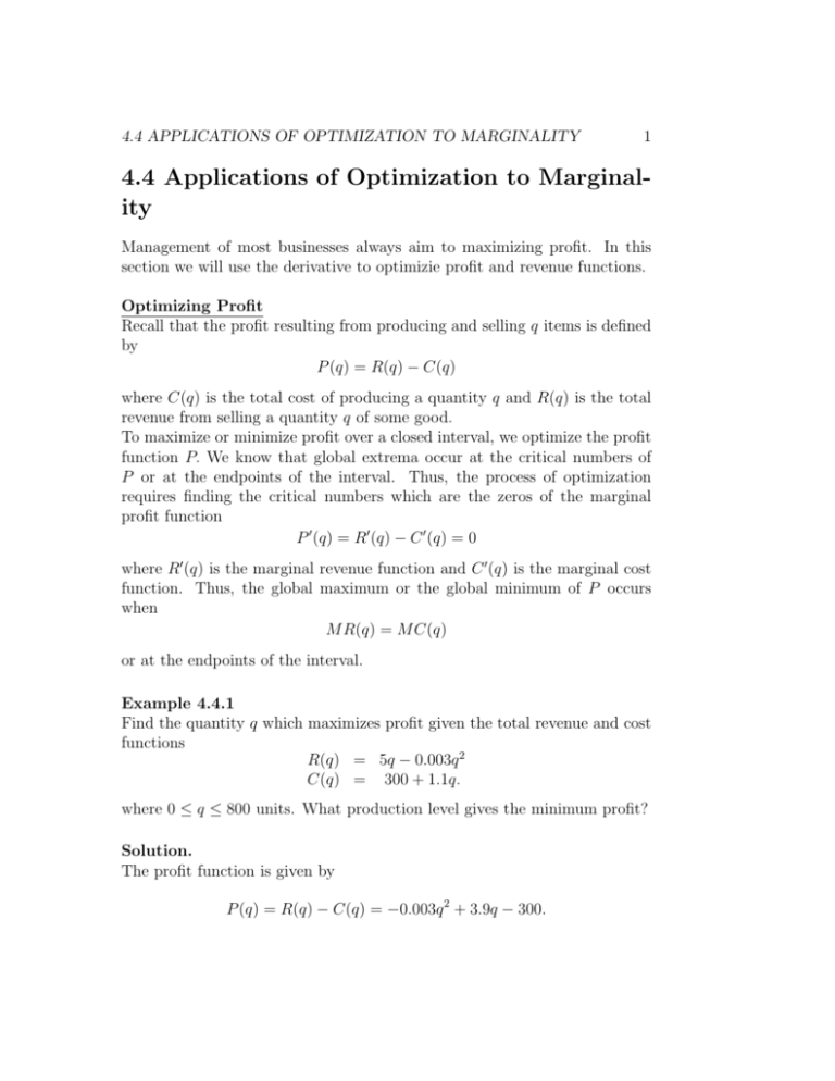
4.4 APPLICATIONS OF OPTIMIZATION TO MARGINALITY
1
4.4 Applications of Optimization to Marginality
Management of most businesses always aim to maximizing profit. In this
section we will use the derivative to optimizie profit and revenue functions.
Optimizing Profit
Recall that the profit resulting from producing and selling q items is defined
by
P (q) = R(q) − C(q)
where C(q) is the total cost of producing a quantity q and R(q) is the total
revenue from selling a quantity q of some good.
To maximize or minimize profit over a closed interval, we optimize the profit
function P. We know that global extrema occur at the critical numbers of
P or at the endpoints of the interval. Thus, the process of optimization
requires finding the critical numbers which are the zeros of the marginal
profit function
P 0 (q) = R0 (q) − C 0 (q) = 0
where R0 (q) is the marginal revenue function and C 0 (q) is the marginal cost
function. Thus, the global maximum or the global minimum of P occurs
when
M R(q) = M C(q)
or at the endpoints of the interval.
Example 4.4.1
Find the quantity q which maximizes profit given the total revenue and cost
functions
R(q) = 5q − 0.003q 2
C(q) = 300 + 1.1q.
where 0 ≤ q ≤ 800 units. What production level gives the minimum profit?
Solution.
The profit function is given by
P (q) = R(q) − C(q) = −0.003q 2 + 3.9q − 300.
2
The critical numbers of P are the solutions to the equation P 0 (q) = 0. That
is,
3.9 − 0.006q = 0
or q = 650 units. Since P (0) = −$300, P (800) = $900 and P (650) = $967.50,
the maximum profit occurs when q = 800 units and the minimum profit(or
loss) occurs when q = 0, i.e. when there is no production
Example 4.4.2
The total revenue and total cost curves for a product are given in Figure
4.4.1.
Figure 4.4.1
(a) Sketch the curves for the marginal revenue and marginal cost on the
same axes. Show on this graph the quantities where marginal revenue equals
marginal cost. What is the significance of these two quantities? At which
quantity is profit maximum?
(b) Graph the profit function P (q).
Solution.
(a) Since R is a straight line with positive slope, its derivative is a positive
constant. That is, the graph of the marginal revenue is a horizontal line at
some value a > 0. Since C is always increasing, its derivative M C is always
positive. For 0 < q < q3 the curve is concave down so that M C is decreasing.
4.4 APPLICATIONS OF OPTIMIZATION TO MARGINALITY
3
For q > q3 the graph of C is concave up and so M C is increasing. Thus, the
graphs of M C and M R are shown in Figure 4.4.2.
Figure 4.4.2
According to the graph, marginal revenue equals marginal cost at the values
q = q1 and q = q2 . So maximum profit occurs either at q1 , q2 or at the
endpoints. Notice that the production levels q1 and q2 correspond to the two
points where the tangent line to C is parallel to the tangent line to R. Now,
for 0 < q < q1 we have M R < M C so that P 0 = M R − M C < 0 and this
shows that P is decreasing. For q1 < q < q2 , M R > M C so that P 0 > 0
and hence P is increasing. So P changes from decreasing to increasing at
q1 which means that P has a minimum at q1 . Now, for q > q2 we have that
M R < M C so that P 0 < 0 and P is decreasing. Thus, P changes from
increasing to decreasing at q2 so q2 is a local maximum for P. So maximum
profit occurs either at the endpoints or at q2 . Since profit is negative for
q < q3 and q > q4 , the profit is maximum for q = q2 .
(b) The graph of P is shown in Figure 4.4.3.
4
Figure 4.4.3
Optimizing Revenue
Example 4.4.3
The demand equation for a product is p = 45 − 0.01q. Write the revenue
function as a function of q and find the quantity that maximizes revenue.
What price corresponds to this quantity? What is the total revenue at this
price?
Solution.
The revenue function is given by R(q) = pq = 45q −0.01q 2 . This is a parabola
that opens down so its vertex is the global maximum. The maximum then
occurs at the critical number of R(q). That is, at the solution of R0 (q) = 0 or
45 − 0.02q = 0. Solving for q we find q = 2250 units. The maximum revenue
is R(2250) = $50, 625. The unit price in this case is p = 45 − 0.01(2250) =
$22.50