Elastic Resources Framework in IaaS, preserving
performance SLAs
Keywords-Clouds, Elasticity, Forecasting, Cost function, Quality of Service.
I. I NTRODUCTION
Elasticity is a key characteristic of the cloud, enabling users
to acquire and relinquish the resources dynamically. In the
current IaaS cloud systems, the resources are provided in the
form of virtual machines (VMs). To acquire more resources,
a cloud user needs to migrate its application to another VM
with more resources, and vice versa. For example, Amazon
provides few standard types of VMs [1] with some predefined configuration like small, medium, and big instance,
and some job specific instances like high memory, high CPU,
high I/O instances. Such provisioning is useful for workloads
whose resource requirements or usage matches the allocation.
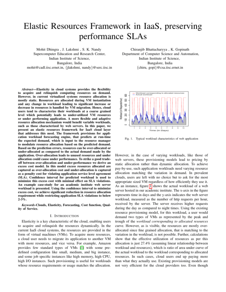
Workload (in Requests/hour)
Workload corresponding to allocated resources
Actual workload
100 200 300 400 500 600
Abstract—Elasticity in cloud systems provides the flexibility
to acquire and relinquish computing resources on demand.
However, in current virtualized systems resource allocation is
mostly static. Resources are allocated during VM instantiation
and any change in workload leading to significant increase or
decrease in resources is handled by VM migration. Hence, cloud
users tend to characterize their workloads at a coarse grained
level which potentially leads to under-utilized VM resources
or under performing application. A more flexible and adaptive
resource allocation mechanism would benefit variable workloads,
such as those characterized by web servers. In this paper, we
present an elastic resources framework for IaaS cloud layer
that addresses this need. The framework provisions for application workload forecasting engine, that predicts at run-time
the expected demand, which is input to the resource manager
to modulate resource allocation based on the predicted demand.
Based on the prediction errors, resources can be over-allocated or
under-allocated as compared to the actual demand made by the
application. Over-allocation leads to unused resources and under
allocation could cause under performance. To strike a good tradeoff between over-allocation and under-performance we derive an
excess cost model. In this model excess resources allocated are
captured as over-allocation cost and under-allocation is captured
as a penalty cost for violating application service level agreement
(SLA). Confidence interval for predicted workload is used to
minimize this excess cost with minimal effect on SLA violations.
An example case-study for an academic institute web server
workload is presented. Using the confidence interval to minimize
excess cost, we achieve significant reduction in resource allocation
requirement while restricting application SLA violations to below
2-3%.
Chiranjib Bhattacharyya , K. Gopinath
Department of Computer Science and Automation,
Indian Institute of Science,
Bangalore, India
{chiru, gopi}@csa.iisc.ernet.in
0
Mohit Dhingra , J. Lakshmi , S. K. Nandy
Supercomputer Education and Research Center,
Indian Institute of Science,
Bangalore, India
mohit@cadl.iisc.ernet.in, {jlakshmi, nandy}@serc.iisc.in
1
2
3
4
5
6
7
8
9
10
Time (in Days)
Fig. 1.
Typical workload characteristics of web application
However, in the case of varying workloads, like those of
web servers, these provisioning models lead to pricing by
static allocation rather than dynamic allocation. To achieve
pay-by-use, such application workloads need varying resource
allocation matching the variation in demand. In prevalent
clouds, users are left with no choice but to ask for the most
appropriate sized VM regardless of how efficiently they use it.
As an instance, figure 1 shows the actual workload of a web
server hosted in our academic institute. The x-axis in the figure
represents time in days and the y-axis indicates the web server
workload, measured as the number of http requests per hour,
received by the server. The server receives higher requests
during the day as compared to night times. Using the existing
resource provisioning model, for this workload, a user would
demand two types of VMs as represented by the peak and
trough of the workload corresponding to allocated resources
curve. However, as is visible, the resources are mostly overallocated since fine grained allocation, that is matching to the
variation in the workload, is not possible. Further, calculations
show that the effective utilization of resources as per this
allocation is just 27.4% (assuming linear relationship between
workload and resources), which is ratio of area under curve of
the actual workload to the workload corresponding to allocated
resources. In such cases, cloud users end up paying more
than what they actually use. Existing provisioning models are
not very efficient for the cloud providers too. Even though
Cloud OS
Tools
Core
Administrator
tools
Information
manager
VM
Manager
Drivers
Service
manager
Accounting
and auditing
Cloud
interfaces
Scheduler
Authorization
and
authentication
Forecasting engine
based on cost model
Network
manager
Image
manager
Storage
manager
Cloud
drivers
Physical infrastructure drivers
Physical Infrastructure
Fig. 2.
Federation
manager
External Clouds
Elastic Resources Framework for IaaS
there are idle resources available, the provider can not release
them for better usage. Inefficient models thus contradict the
whole idea of achieving high server utilization using cloud
computing.
For the workloads described, the current provisioning models ensure preservation of application SLAs, but result in
significant idle resources. To address this gap, in this paper,
we modify the IaaS architecture as shown in Figure 2. The
picture depicts a modified OpenNebula(http://opennebula.org/)
IaaS architecture. To enable fine-grained elasticity, we propose
the Forecasting engine based on cost model depicted in black
color in the core layer of IaaS architecture. By addition of
this component, changes are anticipated in other components
of the architecture, which is captured by gray color boxes.
Other components that are not affected are the white colored
boxes. In the existing IaaS architecture, Scheduler (in Tools)
interacts with VM Manager (in Core) to deploy or reallocate
the VM on the selected server. We introduce a component
Forecasting engine based on cost model into the architecture,
which basically forecasts the resource requirement based on
the history of the application workload that the VM hosts.
It provides fine grained resource requirements to the VM
Manager, which in turn, either fulfills the demand on the same
server or interacts back with Scheduler if it is not possible to
fulfill the demand locally. The component Information Manager which monitors the resource utilization in the VMs, now
also collects and interprets the workload history saved in VM
and presents it to the forecasting engine [2]. The forecast made
by the prediction engine may not be always correct, therefore
leading to under-allocation or over-allocation of resources.
Over-allocation leads to under utilization of resources and
under-allocation leads to poor performance of the application.
To assess the same, we derive an excess cost model and
formulate the problem into a cost optimization problem. The
excess cost comprises of two components, namely, cost due
to over-allocation of resources (COver−allocation ) and the
penalty cost (CSLApenalty ) corresponding to poor application
performance resulting from under-allocation of resources. The
goal of optimization problem is to reduce the excess cost. The
basic intuition of this cost model is to reduce the resource
cost of the user by enabling resource allocation closer to what
is actually used, without compromising on the application
performance. At the same time, by adaptively allocating resources as dictated by the workload, the provider is aware of
idle resources that could potentially be used for some other
workloads. This leads to better utilization of resources.
The main contribution of the paper are as follows:
• A generic fine-grained elastic resources framework for
IaaS cloud based on an excess cost model.
• Finding optimal trade off between over-allocation cost
of resources and under-allocation SLA penalty, using
optimal value of confidence interval of the forecast.
• While leaving the resource provisioning decisions to the
provider, this paper shows how the users’ interest can be
protected by enabling performance based SLAs.
• This paper shows that significant reduction in the resource
allocation can be achieved using dynamic allocation of
resources along with negligible SLA violations, for an
elastic workload. For our case study, we see a reduction
of more than twice in the resource allocation while
restricting application SLA violations to below 2-3%.
The rest of the paper is organized as follows. Section II
provides the motivation for the modification in IaaS cloud
architecture. Section III starts with some definitions and illustrates proposed system model. Section IV explains system
components with the help of a case study and improvement as
a reduction in the resources allocated. Finally, related work is
discussed in section V followed by conclusion in section VI.
II. M OTIVATION FOR MODIFIED I AA S ARCHITECTURE
Elasticity is a property the IaaS layer can provision, if the
application is able to make variable resource requirements.
However, tracking the variability in resource requirement is a
non-trivial problem. Well known approaches to this problem
look at historical data to derive usage patterns. Based on the
past usage characteristics, models are generated to predict
future usage. It is true that prediction models are highly
sensitive to usage patterns of individual applications. Hence,
one would tend to argue the justification of the forecasting
engine into the IaaS layer, which would normally be managed
by the cloud provider.
The issue with forecasting of application workload is that,
over-allocation of resources is a cost on the cloud user, since
pricing is based on allocated resources and under-allocation
(which leads to under performance of application) is a penalty
on the cloud provider, if application is bound by a performance
SLA. A trade off between these two objectives leads to an
optimal situation for both cloud provider and user.
Building application specific forecasting engine may be
a challenge for an application developer. However, if the
IaaS framework provides for some standard forecast engines
like ARIMA(Autoregressive and Integrated Moving Average)
models [3] (explained in detail in section IV-A), many applications stand to benefit. We envisage that the cloud user
would provide the necessary data required by the forecasting
engine to enable building of the model. And subsequently, the
The IaaS cloud layer is the operating system of the cloud
data center. One example of IaaS cloud system is OpenNebula.
Figure 2 gives the architecture overview of OpenNebula IaaS
software, depicting different layers and corresponding components in each layer. Complete description and functional
responsibilities of these layers and components is detailed
in [4]. We introduce the forecasting engine into the core layer
of the OpenNebula architecture. As indicated earlier, the main
function of this component is to host a prediction model for an
application hosted inside a VM on the cloud. While building
this engine, it is important to identify some key application
metrics that are defined as follows:
1.0
0.8
0.6
0.4
SLA Penalty
0.2
III. S YSTEM M ODEL
0.0
IaaS layer would use this model to adjust resource allocations
based on the history of usage by the application. Although the
effort required in building and using the forecasting engine is
not trivial, the benefits do outweigh the efforts involved.
0
500
1000
2000
3000
Response Time (in ms)
Fig. 3.
SLA Penalty function
Workload (Request rate in form of time series)
Time series analysis
and modeling
Find optimal
confidence interval
Model
Confidence Interval
Forecast request rate with bounds
based on confidence interval
Request rate forecast
A. Metrics used
In this study, we consider the case of I/O workloads as
they contribute to latency as perceived by users. In such
applications, we define the workload by the metric Request
rate, the number of requests per unit time; here the number
of requests per hour as we take the scheduling decisions on a
per hour basis. The performance metric that is of interest to
the user is the Response time that the server takes to service
these requests. We use average response time limits to identify
SLA violations, which are captured by SLA penalty functions.
Although the Performance SLA penalty functions are defined
theoretically by many researchers [5], they are not commonly
used, yet, in practice. Figure 3 shows an example of penalty
function which we use, where penalty starts increasing when
the response time increases beyond a threshold (100 ms in our
case) specified in the SLA. It saturates after a point, which
captures a state wherein the response time is so huge that the
service is meaningless to the user. Also, by limiting the penalty
function beyond the saturation point, the cloud provider will
not incur extraordinary losses.
Further, in order to derive the resource requirements from
the request rate, a provider needs some initial information from
the user about the workload hosted in the cloud, for example,
resource requirements of the application that he wants to host,
on the IaaS cloud, to support different request rates. Resource
requirements can be derived using a monitoring framework
described in [6].
B. Proposed Framework
The key component in the proposed elastic resources framework is the forecasting engine which uses an excess cost
model to arrive at an optimal resource allocation based on
predicted workload for the application. The forecast engine
uses associated confidence intervals for the predicted workload
to optimize the resource allocation. Figure 4 details the component Forecasting Engine based on cost model discussed in
the Figure 2. The input to the engine is the user workload and
Derive resource requirement
based on upper bound of forecast
Resource Derivation
Logic
Resource requirement
Fig. 4.
Forecasting engine based on Cost Model
it outputs the optimal resource requirements. The forecasting
engine uses past history of the application workload and builds
a time-series model out of it. Systematic analysis of the
time series is executed offline to build a prediction model. A
probabilistic bound of the forecast, within a given confidence
interval, is generated using the prediction model. For instance,
upper and lower bounds of the forecast for 95% confidence
interval implies that the probability that the forecast would
be within the upper and lower bounds is 0.95. We use the
upper bound of the forecast to provision the resources since
we also want to minimize the SLA violations. By increasing
confidence interval, over-allocation cost will increase and SLA
violations penalty will decrease. Hence, confidence interval is
the key to control the two excess cost functions associated
with the allocation.
Finding Optimal Confidence Interval: The optimal confidence interval is based on the minimization of the total excess
cost of the system. Mathematically, if CExcess defines the excess cost, which is defined as a function COver−allocation and
CSLApenalty , then the optimization problem can be formulated
as follows:
M inimize
CExcess = COver−allocation (α) + CSLApenalty (α) (1)
subject to
0 < α < 100
(2)
where, α is the confidence interval. Both COver−allocation
and CSLApenalty are functions of confidence interval. The
Workload in form of time series
Confidence
Interval
Training
Data
Test
Data
Resource Derivation
Logic
Calculate
Response time
Calculate SLA
Penalty Cost (C1)
Derive actual
Resource requirement
Calculate
over−allocation cost (C2)
Total Cost = Total Cost + C1 + C2
More Test Data ?
Yes
No
Total Cost
Find optimal confidence interval to minize total cost
Optimal Confidence Interval
Fig. 5.
Finding Optimal confidence interval
solution to this optimization problem would give us the
optimal value of confidence interval, which a provider can
choose to minimize the excess cost.
Figure 5 further describes the component Find optimal
confidence interval discussed in the Figure 4. First of all, we
split the data into two parts: training and test data. Using the
training data, a model is built and we derive the resources
using the same Resource Derivation Logic used in Figure 4.
Then, based on the resources allocated by the forecast and
the actual workload, we check the response time of the
system. If the response time of the system exceeds a threshold
defined in SLA, we calculate SLA penalty cost based on
SLA penalty function. Otherwise, we compare the predicted
resources with the resources actually required, and calculate
the over-allocation cost. Excess cost is the sum of these two
costs for all of the test points. For each point, we need to
update the model to include the next test point. Note that
update does not mean recalculation of model parameters every
time. Then, we update the confidence interval and repeat the
procedure again to find excess cost, and the objective is to
reach to a point near to optimal confidence interval, where
excess cost is minimized. We describe the components in detail
with the help of a case study in the following section.
IV. C ASE S TUDY
To illustrate a use case, we analyze the workload of the
web server hosted in our academic institute. Web servers
are one of the most popular I/O workloads that are getting
hosted on cloud systems [2]. These workloads can benefit from
inherently elastic resource provisioning.
A. Time Series Analysis and Modeling
To analyze the workload using a time-series model we
capture the request rate variations, hitting the web server,
in the form of a discrete time series. We observe that this
request rate series has a seasonal trend of 24 hours, except
for the weekends. Hence, we first separate the time series into
data corresponding to weekdays and another corresponding to
weekends. The case study described below uses the weekdays
data only, which was depicted as Actual Workload in Figure 1.
Normally, web applications hosted on cloud are multi-tier
(consisting of different components in different VMs). In that
case, it would represent the workload of front-end component.
The weekends data will have a similar model and is not
described in the paper. But the final model will have both
these incorporated. As discussed earlier, each point represents
the total number of requests for one hour. For our workload the
request rate is captured on an hourly basis, hence we assume
the scheduling decisions would be taken at the interval of one
hour, and thus it makes sense to forecast the request rate for
next one hour.
For the modeling of time series and prediction, we use
Seasonal ARIMA (SARIMA) model. To illustrate the same,
we first introduce basic ARMA model. ARMA model includes
two components : a) Autoregressive - regression on itself, that
is, the current value of the series x(t) can be explained as a
function of p past values x(t − 1), x(t − 2), ... , x(t − p) and
p is the number of steps into the past needed to forecast the
current value, b) Moving-average model where in the current
value of the series is explained in terms of previous q white
noise terms w(t−1), w(t−2), ..., w(t−q) , that is, past q white
noise terms are combined linearly to form the observed data1 .
Mathematically, ARMA model can be represented as,
x(t) = w(t) +
p
X
q
X
φi x(t − i) +
i=1
θi w(t − i)
(3)
i=1
Autoregressive term
Moving-average term
where, φi is the coefficient of the x(t − i), θi is the coefficient
of the w(t−i). It is easy to represent the above equation using
a backward operator B. It is defined as,
B(x(t)) = x(t − 1),
B 2 (x(t)) = x(t − 2) and so on.
The equation 3 can be rephrased as following :
x(t) = w(t) +
p
X
φi B i (x(t)) +
i=1
=⇒ (1 −
p
X
φi B i )x(t) = (1 +
i=1
=⇒ φp (B)x(t) = θq (B)w(t)
q
X
θi B i (w(t))
(4)
i=1
q
X
θi B i )w(t)
(5)
i=0
(6)
where, φp and θq are AR and MA functions of order p and q
respectively. That is,
φp (B) = 1 − φ1 B − φ2 B 2 ... − φp B p , and similarly
θq (B) = 1 + θ1 B + θ2 B 2 ... + θq B q .
The basic assumption in ARMA models is that the process
x(t) is stationary2 . If a process is not stationary , then
1 White Noise series is a sequence of uncorrelated random variables with
zero mean and finite variance.
2
Stationary process is the one whose mean does not change with time and
covariance depends on the time lag and not absolute time.
Request Rate (Requests/hour)
(7)
where, (1 − B)x(t) = x(t) − x(t − 1), which basically
implies the differencing of x(t). We may have to perform
the differencing a number of times to obtain the stationarity,
which is why the differencing operator (1 − B) may have to
be applied d times.
Finally, seasonal ARIMA is an extension of ARIMA model
to include seasonal components, which capture the seasonal
variations in the series. The seasonal part of an SARIMA
model has the same structure as the non-seasonal one in
ARIMA: it may have an AR factor, an MA factor, and an
order of seasonal differencing. Mathematically, the model can
be represented as :
ΦP (B S )φp (B)(1 − B S )D (1 − B)d x(t) = ΘQ (B S )θq (B)w(t)
(8)
where, ΦP (B S ) and ΘQ (B S ) are the AR and MA polynomials of seasonal part, and (1 − B S ) is the difference operator
with a seasonal difference lag S, that is, (1 − B S )x(t) =
x(t − S). In our case, this seasonal lag is 24 hours. To model
seasonal component, we first take the difference of the series
with a difference interval of 24 hours. Or, in other words,
if x(t) denotes the weekdays time series, then the difference
series is x(t) − x(t − 24). This difference series is stationary
(confirmed by very low p-value = 0.01 in Augmented DickeyFuller Test, which shows that we can reject the null hypothesis
that the series is non-stationary), and hence we can use the
SARIMA model for our data.
To find the number of parameters of the model, that is, the
number of steps into the past, needed to predict the current
value, we rely on AIC (Akaike information criterion). AIC is a
measure of relative goodness of fit of different models to the
observed data. It provides a nice tradeoff between accuracy
and complexity of the model. Preferred model among all of
the models is the one with minimum AIC value. In our case,
using the above criterion, we find out the optimal number
of parameters and coefficients using forecast package [7] in
R. For our case, the model parameters that best describe the
model are : p=1, d=0, q=1, P=0, D=1, Q=1, S=24. After
finding the coefficients, the equation governing the system for
our time series workload comes out to be following :

T 

0.7231
x(t − 1)


 x(t − 24) 
1




−0.7231
 x(t − 25) 




 ×  w(t) 
1
x(t) = 
(9)




 0.5445 
 w(t − 1) 




 0.9465 
w(t − 24)
0.5154
w(t − 25)
0
φp (B)(1 − B)d x(t) = θq (B)w(t)
100 200 300 400 500 600 700
sometimes differencing a series helps to make the process
stationary. ARIMA model is an extension of ARMA, where
the series x(t) is assumed to be an integrated process (which
on differencing becomes stationary) , and so in ARIMA model,
instead of x(t), a difference series is used. For ARIMA, the
model can be described as follows :
Original workload
Predicted (alpha = 0%)
o Predicted (alpha = 75%)
Predicted (alpha = 99.5%)
●
●
●
●
●●
●●
●
●
●
●
●
●
●
●
●●
●
●
●
●
●
●
●
●
●●
●
●
●
●
●
●
●●
●
●
●
●
●
●
●
●
●
●
●
●
● ●
●
●●
●
●
●
●● ●
● ●●
●●
●
●
●
●
●●
●
●
●
●
●● ●
●
●●
● ●●
●
● ●
●
●
●
●
●
● ● ●
●
●
●
●● ●
●●
●
●
●
●
● ●● ● ●
●● ●
●
●
●
●
●
● ● ●
●● ● ●
●
●
● ●● ●
●
●
● ● ●
●
●
●
●
●
●
● ●
●
●
●
●
● ●●
●
●
●● ●
●● ●
● ●
●● ●
●
●
●
●
●
●
●
●
●
●
●
●
●
●
●
●
●
●
●
●●
●
●
● ●
●
●
●
●
●
●
●
●
●
●
●
●
●
●
●
●
●
●
●
●
●
●
●
●
●
●
●
●
●
●
●
●
●
●
●
●
●
●
●
●
●
●
●
●
●
●
●
●
●
●
●
●
0
100
200
300
400
Time (in hours)
Fig. 6.
Forecast with actual data
Furthermore, we observe that the autocorrelation of the residuals of the predicted data is almost zero. This indicates that
the model is correctly specified with no bias [3].
B. Forecasting
To forecast the demand, we use the model generated above
to predict within a confidence interval. For the first time, an
initial value of the confidence interval is specified as the input.
After that, it is provided as a feedback to minimize the excess
cost of the system. In this study, 240 observations are used
to construct the model and it is forecasted and tested for the
next 240 observations. Figure 6 shows the forecast based on
the model constructed above. Solid line shows the observed
values, and the upper bound of the forecast using different
confidence intervals is shown. 0% confidence interval implies
the actual forecast with no bounds. As the confidence interval
is increased, the upper bound of the forecast moves upwards.
C. Deriving Resource Requirements
To derive resource requirements for the observed data,
we use the web server logs to synthesize workload on an
experimental cloud set up. In the experimental setup, web
server is hosted on a VM. OpenNebula cloud is used to
build the IaaS cloud with KVM 3 as hypervisor. In order
to generate the http requests, we use httperf [8] as a client
program. Along with generating varying http requests, it also
has other capabilities like measuring average response time
and throughput, which would help us evaluating our model
in the later steps. We run our experiments on an AMD 2.4
GHz system having 12 cores and 16 GB memory. Figure 7
shows the variation of VM CPU usage with request rate. As
expected, CPU requirement of VM increases with increase in
request rate [9]. We use this to derive the resources required
to support a given workload (request rate).
D. Provisioning Resources
The forecasted request rate can be used to provision the
infrastructural resources. In our study, we provision the VM
CPU and let the other resources (like memory, network
3
Kernel based Virtual Machine (http://www.linux-kvm.org)
Request Rate - 100
Request Rate - 200
Request Rate - 300
Request Rate - 400
Request Rate - 500
Request Rate - 600
Request Rate - 700
20
30
Response Time (in ms)
40
3000
10
VM CPU Requirement (in percent)
3500
2500
2000
1500
1000
500
0
100
200
300
400
500
600
700
Request Rate (Requests/hour)
0
0
Fig. 7.
10
20
Resource Requirement
35
Fig. 9.
30
40
50
60
70
VM CPU Allocated
80
90
100
Response time with varying request rates and CPU allocated
20
25
P
|Xt − X̂t |
SM AP E = P
Xt + X̂t
●
●
●
●
●
●●
●
●●
●● ●
●●
●
●
●●
●
●
●
●
●
●
●
●
●
●
●
●
●
●
●
●
●
●
●
●
●
●
●
●
●
●
●
● ●
●
●
●
●● ●
●
●
●
●
● ●
●
●
●● ●
●
●
●● ●
●
●
●
● ●
●
●
●
●●
●
●
●
●
●
● ●
●
●
●
●
●
● ●●
●● ● ●
●
●
●
●
●
●●●
● ●
●
●
●
●
●
●
●
● ●
●●
●
●
●
● ●
●
●
●
●
● ●
●
●
●
●
●
●
●
●● ●
●
●
●
●● ●
●
●
● ●
● ● ●
● ●
●●
●
●
●
●● ●●
●
●
●
●
●
●
●
●
●
●
●
●
●● ● ● ●
●
●
●
●
●
●
●
●
●
●
●
●
●
●
●
●
●
●
●
●
●
●
●
●
●
●
●
●
●
●
●
●
●
●
●
●
●
●
●
●
●
●
●
●
●
●
●
15
10
5
0
CPU Requirement (in percent)
30
is defined as follows:4 :
●
●
●
●
●
●
●
●
●
●
●●
Actual CPU requirement
Predicted (alpha = 0%)
o Predicted (alpha = 75%)
Predicted (alpha = 99.5%)
●
0
100
200
300
400
(10)
where, Xt is the actual CPU requirement and X̂t is the
predicted CPU requirement. For our case, the value of SMAPE
for the actual CPU requirement prediction (0% confidence
interval) has come out to be 6.67071%, which is quite good
and shows the credibility of our approach.
Time (in hours)
Fig. 8.
Predicted vs Actual CPU requirement
bandwidth) be unconstrained. Based on the variation of VM
CPU with request rate as mentioned in Figure 7, we calculate
the CPU requirement using interpolation. We round off the
request rate to the nearest multiple of 50 requests/s, and the
corresponding VM CPU to the nearest multiple of 2%. For
example, if the VM CPU requirement has been derived to be
16.9%, we allocate 18% of the CPU. Also, using the actual
request rate values, we calculate the actual VM CPU that is
required, such that the response time of the system stays within
the defined limits. Figure 8 shows the comparison of the actual
and predicted VM CPU requirement, based on the earlier
forecast of the request rates. Again, based on the different
confidence intervals of the bound of the forecast on request
rate, VM CPU requirements are derived as shown in the figure.
Since the VM CPU requirements is almost linear with respect
to request rate, forecast of CPU requirement is on the similar
lines to that of forecast of request rate, but has discrete values
of CPU because of the rounding off.
Performance Measure of Resource Provisioning: We forecast the request rate and use it to derive the resources for allocation. Provisioned resources dictate the system performance.
Hence,forecast accuracy is measured in terms of resource
requirement against allocation. Several performance metrics
have been proposed in literature to measure forecast accuracy.
In this paper, we use an absolute percentage accuracy measure,
SMAPE (Symmetric mean absolute percentage error). SMAPE
E. Calculate Response Time
Response time is used to measure SLA violations, as
mentioned earlier. In order to derive the response time of the
system, we use a) provisioned resources (VM CPU) based
on prediction and, b) the actual request rate. In other words,
we need to find how does the system behave if we allocate
the resources based on prediction. To find this, we conduct
experiments by providing limited resources to the system
and measure the response time of the system. We limit the
CPU allocated to the VM and vary the limit from 0 to
100% for different request rates. Figure 9 shows the response
times observed at different request rates, when we limit the
CPU from 2% to 100%. We notice that response time starts
decreasing and comes under the defined performance SLA
limit (where SLA violations do not occur, it is 100 ms as per
Figure 3), after a certain point . For example, at the request
rate of 200, response time is well under 100 ms after 14% of
VM CPU. We call this point as Safe Resource Allocation Point
(SRAP). This SRAP increases with increase in the request rate
as can be observed from the Figure 9.
Next, we calculate the value of response time for our
simulated web server workload using the resources allocated,
and the actual request rate. Figure 10 shows the behavior of
the response time corresponding to the resources allocated
(corresponding to 0% confidence interval). Dotted line denotes
the safe response time for the system, and all of the points
where the response time exceeds the safe limit correspond to
SLA violation points.
4
http://en.wikipedia.org/wiki/Symmetric mean absolute percentage error
600
400
0
200
Workload (in Requests/sec)
6
4
2
SLA Violations Limit
Response Time
based on prediction
0
Response Time (logarithmic plot) in ms
Allocation using our framework
Actual workload
Static Allocation
0
100
200
300
400
1
2
3
Time (in hours)
Response time of system for the allocated resources
Fig. 12.
6
7
8
9
10
Reduction in resource allocation
0.0
Indicates Minima
0
20
40
60
10
0
Actual required resources allocation
Static Allocation
Predicted resources allocation
−30
0.000125
0.00025
0.0005
−10
Rate of change of resources
SLA Penalty slope for response time
−20
0.4
0.6
0.8
Over−allocation cost factor for CPU = 0.002
0.2
Excess Cost Function
5
20
1.0
Fig. 10.
4
Time (in Days)
80
100
0
50
Fig. 11.
Excess cost with confidence interval
Excess cost at each point in the time series can be found as
following :
CExcess
150
200
250
Fig. 13.
Rate of change of allocation
G. Improvement using framework
F. Cost function


α ∗ RExcess
= β ∗ RT imeExceeded


0
100
Time (in hours)
Confidence Interval
Over-allocation cost
SLA penalty cost
otherwise
Here, RExcess denotes the extra resources allocated than
required and RT imeExceeded denotes the response time of the
system that exceeded beyond threshold defined in SLA. α and
β are the weights for the two cost functions. Total excess cost
is the sum of the excess cost calculated at each point. As we
discussed, the cost functions described above are the functions
of confidence interval. The objective is to find the minimum
excess cost (or an optimal value of confidence interval).
Figure 11 depicts the variation of excess cost function with
confidence interval for our data using different weights of the
cost. Choosing different value of weights associated with overallocation and SLA penalty cost leads to a different minima.
As can be observed from the figure, by increasing β, the
optimal confidence interval increases. At higher confidence
interval, SLA violations will be less and over-allocation of
resources will be more. In this way, one can prioritize SLA
violations over over-allocation and vice-versa based on the
user’s requirement.
Figure 12 shows the predicted workload using the confidence interval which minimizes the excess cost (using β =
0.00025). As can be seen, it forms an approximate envelope
over the original workload. We also find reduction in the
resource allocation when we use our framework than when
we do a static allocation. Actual workload needs just 27.4%
of the resources of the static allocation, as stated earlier. In
static allocation case, the allocated resources are 3 times more
than what is required. Now, using our framework, the allocated
resources are just 1.5 times of the required ones. Thus we get
an improvement of more than twice in the resource utilization
efficiency. Also, using this allocation, the SLA violations occur
for just 2.5% of the workload. It depends on the pricing policy
and SLA penalty, to choose the appropriate cost.
Further, figure 13 shows the rate of change of resources
allocated for three different scenarios : actual resources that are
required for the given workload, static allocation as depicted
in figure 2, predicted resource allocation as provided by the
framework. Rate of change of predicted resources is more
close to the rate of change of actual resources, than the static
one. The more close the change of allocation is to the change
of actual resources required, more elastic is the resource
allocation framework. The quantification of the elasticity is
beyond the scope of this paper and is left as a future work.
The elasticity metric could then be used as a discriminator
to understand whether the proposed framework would give
significant improvement over static allocation or not.
V. R ELATED W ORK
In this work, we have proposed a novel framework of
providing fine-grained elasticity for IaaS cloud. To the best
of our knowledge, no one has approached the problem of
dynamic provisioning by way of finding an optimal tradeoff
between the over-allocation and under-allocation using a cost
model. We look at our related work with respect to elasticity
and revenue maximization in clouds.
Extensive literature belongs to a category of reactive schedulers. In [10], Fito et. al. have developed an SLA-aware
resource manager, which aims to maximize the revenue of
cloud provider. Based on the immediate state of the system,
they provision the appropriate amount of resources. However, it would not capture the trend in the workload, which
our framework captures using SARIMA model. In [11], a
stochastic model of resources in virtualized environments and
scheduling algorithm are proposed to provide performance
guarantees and aims towards server consolidation. In this
paper and other papers aiming towards server consolidation
in virtual servers, elasticity of the workload is not taken into
consideration. Regarding forecasting strategies, Bobroff et. al.
in [12] have introduced dynamic server migration and consolidation algorithm, wherein they use the periodograms to find
the periodic components in the CPU utilization series. They
demonstrate that variability in the workload accrue the benefits
of dynamic placement of VMs. In our framework, by using
the feedback loop, it would automatically come up with the
most appropriate type of allocation based on the workload. If
the workload has no pattern, it would automatically provision
the resources close to static provisioning. If it is varying
then the framework would choose local provisioning (vertical
scaling) or replicate (horizontal scaling) based on the predicted
workload. Another related work in [13] uses ensemble timeseries prediction method to minimize the number of physical
servers, however performance SLAs are not considered. Gong
et. al in [14] have proposed PRESS (PRedictive Elastic
ReSource Scaling) scheme for cloud systems, where in they
find the most dominating frequency component if there is
significant periodic pattern in the signal, otherwise opt for
Markov model to forecast, and they have stated very good
prediction accuracy. We believe that, we can use any forecasting strategy in our framework, since it is assumed as a
black box component. The better prediction accuracy of the
forecast would further reduce the total excess cost. Hence,
our framework provides an advancement to the state-of-theart systems. Finally, Shen et. al. in [15] have described an
elastic resources scaling framework, which builds upon PRESS
scheme for cloud systems. They use strategies to reduce the
SLA violations by padding an extra amount of resources based
on different scenarios. In our paper, the most appropriate
padding of resources is automatically found using the optimal
confidence interval which minimizes the total excess cost.
Also, instead of forecasting each resource separately (CPU,
memory, etc.), we forecast request rate, which is the true
indicator of workload and is used to derive the resource tuple.
VI. C ONCLUSION
Adaptive provisioning of resources based on variations in
workload, improves the overall resource utilization of the
system. In this paper, we have described an elastic resource
provisioning framework, by capturing the change in workload
demand. The approach to the problem is finding an optimal
trade off between over-provisioning and under-provisioning,
which automatically provides the most appropriate allocation
of the resources based on the workload characteristics. This
framework benefits both cloud user and provider. Also, it
ensures the performance guarantees to the user by restricting
SLA violations to a minimum (2-3%) while significantly
reducing resource allocations.
R EFERENCES
[1] “Amazon EC2 Instance Types,” 2013. [Online]. Available: http:
//aws.amazon.com/ec2/instance-types/
[2] G. Reig and J. Guitart, “On the anticipation of resource demands to
fulfill the qos of saas web applications,” in Grid Computing (GRID),
2012 ACM/IEEE 13th International Conference on, sept. 2012, pp. 147
–154.
[3] R. H. Shumway and D. S. Stoffer, Time Series Analysis and Its Applications (Springer Texts in Statistics). Secaucus, NJ, USA: Springer-Verlag
New York, Inc., 2005.
[4] R. Moreno-Vozmediano, R. S. Montero, and I. M. Llorente, “Iaas
cloud architecture: From virtualized datacenters to federated cloud
infrastructures,” Computer, vol. 45, no. 12, pp. 65–72, 2012.
[5] K. Boloor, R. Chirkova, T. Salo, and Y. Viniotis, “Analysis of response
time percentile service level agreements in soa-based applications,”
in Global Telecommunications Conference (GLOBECOM 2011), 2011
IEEE, dec. 2011, pp. 1 –6.
[6] M. Dhingra, J. Lakshmi, and S. K. Nandy, “Resource usage monitoring
in clouds,” in Grid Computing (GRID), 2012 ACM/IEEE 13th International Conference on, sept. 2012, pp. 184 –191.
[7] R. J. H. with contributions from Slava Razbash and D. Schmidt,
forecast: Forecasting functions for time series and linear models, 2012,
r package version 3.25. [Online]. Available: http://CRAN.R-project.org/
package=forecast
[8] D. Mosberger and T. Jin, “httperf-a tool for measuring web server
performance,” SIGMETRICS Perform. Eval. Rev., vol. 26, no. 3, pp. 31–
37, dec 1998. [Online]. Available: http://doi.acm.org/10.1145/306225.
306235
[9] A. Anand, M. Dhingra, J. Lakshmi, and S. K. Nandy, “Resource usage
monitoring for kvm based virtual machines,” in Proceedings of the
18th annual International Conference on Advanced Computing and
Communications (ADCOM 2012), To Be Published, dec. 2012.
[10] J. Fito, I. Goiri, and J. Guitart, “Sla-driven elastic cloud hosting provider,” in Parallel, Distributed and Network-Based Processing
(PDP), 2010 18th Euromicro International Conference on, feb. 2010,
pp. 111 –118.
[11] C. Jiang, X. Xu, J. Zhang, Y. Li, and J. Wan, “Resource allocation in
contending virtualized environments through vm performance modeling and feedback,” in Chinagrid Conference (ChinaGrid), 2011 Sixth
Annual, 2011, pp. 196–203.
[12] N. Bobroff, A. Kochut, and K. Beaty, “Dynamic placement of virtual
machines for managing sla violations,” in Integrated Network Management, 2007. IM ’07. 10th IFIP/IEEE International Symposium on, 21
2007-yearly 25 2007, pp. 119 –128.
[13] Y. Jiang, C. shing Perng, T. Li, and R. Chang, “Self-adaptive cloud
capacity planning,” in Services Computing (SCC), 2012 IEEE Ninth
International Conference on, 2012, pp. 73–80.
[14] Z. Gong, X. Gu, and J. Wilkes, “Press: Predictive elastic resource scaling
for cloud systems,” in Network and Service Management (CNSM), 2010
International Conference on, oct. 2010, pp. 9 –16.
[15] Z. Shen, S. Subbiah, X. Gu, and J. Wilkes, “Cloudscale: elastic
resource scaling for multi-tenant cloud systems,” in Proceedings of
the 2nd ACM Symposium on Cloud Computing, ser. SOCC ’11. New
York, NY, USA: ACM, 2011, pp. 5:1–5:14. [Online]. Available:
http://doi.acm.org/10.1145/2038916.2038921