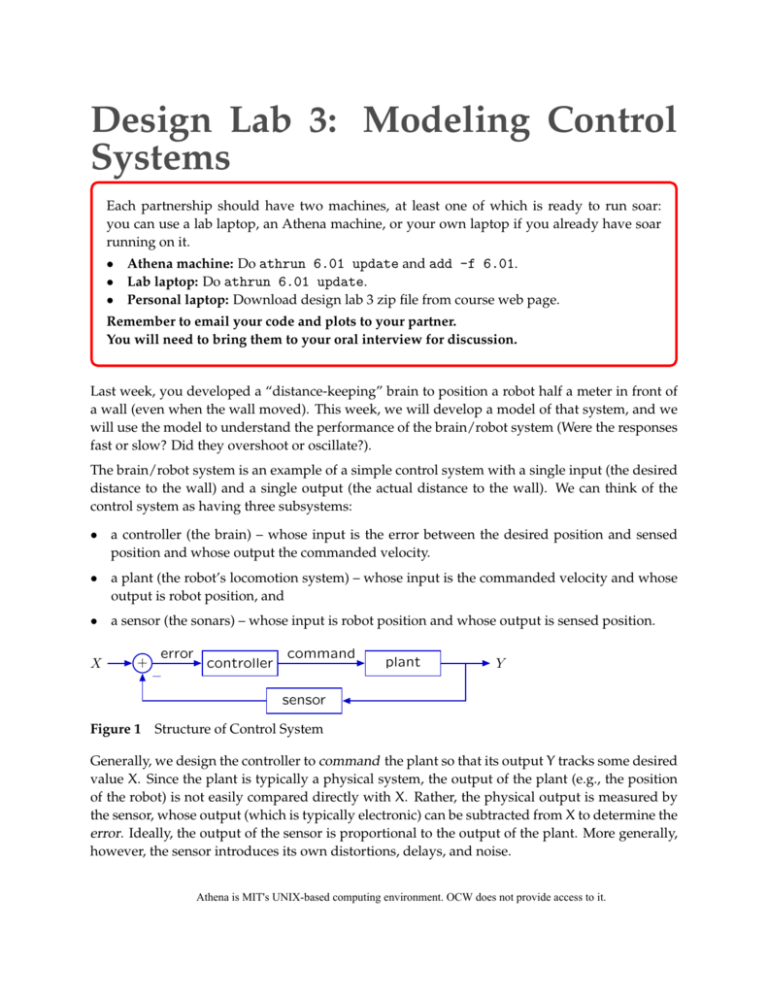
Design Lab 3: Modeling Control
Systems
Each partnership should have two machines, at least one of which is ready to run soar:
you can use a lab laptop, an Athena machine, or your own laptop if you already have soar
running on it.
• Athena machine: Do athrun 6.01 update and add -f 6.01.
• Lab laptop: Do athrun 6.01 update.
• Personal laptop: Download design lab 3 zip file from course web page.
Remember to email your code and plots to your partner.
You will need to bring them to your oral interview for discussion.
Last week, you developed a “distance-keeping” brain to position a robot half a meter in front of
a wall (even when the wall moved). This week, we will develop a model of that system, and we
will use the model to understand the performance of the brain/robot system (Were the responses
fast or slow? Did they overshoot or oscillate?).
The brain/robot system is an example of a simple control system with a single input (the desired
distance to the wall) and a single output (the actual distance to the wall). We can think of the
control system as having three subsystems:
• a controller (the brain) – whose input is the error between the desired position and sensed
position and whose output the commanded velocity.
• a plant (the robot’s locomotion system) – whose input is the commanded velocity and whose
output is robot position, and
• a sensor (the sonars) – whose input is robot position and whose output is sensed position.
X
+
error
−
controller
command
plant
Y
sensor
Figure 1 Structure of Control System
Generally, we design the controller to command the plant so that its output Y tracks some desired
value X. Since the plant is typically a physical system, the output of the plant (e.g., the position
of the robot) is not easily compared directly with X. Rather, the physical output is measured by
the sensor, whose output (which is typically electronic) can be subtracted from X to determine the
error. Ideally, the output of the sensor is proportional to the output of the plant. More generally,
however, the sensor introduces its own distortions, delays, and noise.
Athena is MIT's UNIX-based computing environment. OCW does not provide access to it.
Design Lab 3 — Fall 09
2
1 Difference equations
If we let X be the input signal of a system, and Y be the output signal, then we can describe any
linear time-invariant (LTI) system using a difference equation of the form:
y[n] = c0 y[n − 1] + c1 y[n − 2] + . . . + ck−1 y[n − k] + d0 x[n] + d1 x[n − 1] + . . . + dj x[n − j]
for a fixed set of constants c0 , . . . , ck−1 , d0 , . . . , dj . That is, the output of the system at step n is
a linear combination of some number, k, of samples of the output signal at previous steps, and
some number, j, of samples of the input signal (the sample at step n, and j − 1 previous ones).
Here are some examples:
• Output at step n is 3 times the input at step n: y[n] = 3x[n]
dCoeffs: 3, cCoeffs: none
• Output at step n is the input at step n − 1: y[n] = x[n − 1]
dCoeffs: 0 1, cCoeffs: none
• Output at step n is 2 times the input at step n − 2: y[n] = 2x[n − 2]
dCoeffs: 0 0 2, cCoeffs: none
• Output at step n is 2 times the output at step n − 1: y[n] = 2y[n − 1]
dCoeffs: none, cCoeffs: 2
• Output at step n is the output at step n−1 plus the output at step n−2: y[n] = y[n−1]+y[n−2]
dCoeffs: none, cCoeffs: 1 1
Wk.3.2.1
Do tutor problem Wk.3.2.1.
2 Difference equations for wall finder
Make a simple model of the brain/robot system, as follows. Let Do represent the current dis­
tance from the robot to the wall, and let Di represent the desired distance to the wall. Also let V
represent the forward velocity of the robot. Let T = 0.1 seconds represent the time between steps.
Di
Do
Design Lab 3 — Fall 09
3
Check Yourself 1. Fill in the missing value:
V[0] = 1
Do [0] = 3
V[1] = 2
Do [1] =
Assume the system has the structure shown in Figure 1. Assume that the sensor measures the
current distance Do and generates the sensed distance Ds , which is equal to the current distance
Do delayed by one step time. Let E represent the error signal Di −Ds . On each step, the controller
should command a forward velocity V in proportion to the error so that V = kE. Choose k so
that the velocity is 5 m/s when the desired location is 1 m in front of the robot. Assume that the
robot immediately achieves the commanded velocity when it receives the command and that it
maintains that velocity until it receives the next command.
Check Yourself 2. Fully label the signals (wires) in the following diagram for the brain/robot
system. Include Do , Di , Ds , V , E. Don’t write inside the boxes.
+
−
Determine difference equations to relate the inputs and outputs of
• the controller
• the model of the plant
• the model of the sensor
Combine these equations to derive a difference equation that relates Do to Di .
Design Lab 3 — Fall 09
4
Hint: convert the difference equations to operator equations (with R), solve for Do in terms of
Di , and then convert the result back to a difference equation.
Wk.3.2.2
Enter the coefficients of your difference equations into the tutor, as in­
structed in tutor problem Wk.3.2.2.
3 State machines primitives and combinators
We can build up all linear time-invariant system systems using two primitive state machines:
sm.Gain and sm.R.
The sm.Gain state machine is really just a pure function: the output at step n is the input at step
n, times a constant, k. The state is irrelevant.
class Gain(SM):
def __init__(self, k):
self.k = k
def getNextValues(self, state, inp):
return (state, self.k*inp)
The sm.R state machine is a renamed version of the Delay state machine. It takes a value at
initialization time which specifies the initial output of the machine. Remember that a delay box is
supposed to output its input at the previous time step, but before we start the machine there was
no input, so we need to specify the output at step 0. Thereafter, for n > 0, the output at step n is
the input at step n − 1.
class R(SM):
def __init__(self, v0 = 0):
self.startState = v0
def getNextValues(self, state, inp):
return (inp, state)
Now, we introduce some methods for combining state machines. In cascade composition, we take
two machines and use the output of the first one as the input to the second:
m1
m2
If m1 and m2 are state machines, then you can create their cascade with
Design Lab 3 — Fall 09
5
newM = sm.Cascade(m1, m2)
Now newM is itself a state machine. So, for example, sm.Cascade(sm.R(0), sm.R(0)) will
make a machine that delays by two.
In feedback addition composition, we take two machines and connect them as shown below:
+
m1
m2
Note that the output of m2 is added to the input. If m1 and m2 are state machines, then you can
create their feedback addition composition with
newM = sm.FeedbackAdd(m1, m2)
Now newM is itself a state machine. So, for example, newM = sm.FeedbackAdd(sm.R(0),
sm.Gain(1)) makes a machine whose output is the sum of the inputs from step 0 up to but
not including the present step. You can test it by feeding it a sequence of inputs; in the example
below, it is the numbers 0 through 9:
>>> newM.transduce(range(10))
[0, 0, 1, 3, 6, 10, 15, 21, 28, 36]
Feedback subtraction composition is the same, except the output of m2 is subtracted from the
input, to get the input to m1. (Note the minus sign next to the output of m2 as it’s fed into the
adder.)
+
−
m1
m2
Note that if you want to apply one of the feedback operators in a situation where there is only
one machine, you can use the sm.Gain(1.0) machine, which is essentially a wire, as the other
argument.
Check Yourself 3. Use gains, delays, and adders to draw a system diagram for the first system in tutor problem Wk.3.2.1.
Design Lab 3 — Fall 09
Check Yourself 4. Use gains, delays, and adders to draw a system diagram for the second
system in tutor problem Wk.3.2.1.
Check Yourself 5. Use gains, delays, and adders to draw a system diagram for the third sys­
tem in tutor problem Wk.3.2.1.
Wk.3.2.3
Do tutor problem Wk.3.2.3
Check Yourself 6. Use gains, delays, and adders to draw system diagrams for the controller
in the wall-finder system.
6
Design Lab 3 — Fall 09
Check Yourself 7. Use gains, delays, and adders to draw system diagrams for the plant in the
wall-finder system.
Check Yourself 8. Use gains, delays, and adders to draw system diagrams for the sensor in
the wall-finder system.
Check Yourself 9. Connect the previous three component systems to make a diagram of the
wall-finder system; refer to Figure 1, draw a box around each of the con­
troller, plant and sensor models.
Checkoff 1.
Show your system diagrams to a staff member. Identify the instances of
cascade and feedback composition for the wall-finder system.
7
Design Lab 3 — Fall 09
Wk.3.2.5
8
Do tutor problem Wk.3.2.5
With a value of T = 0.1 and an initial distance to the wall of 1.5 meters, experiment with different
values of the gain. You can do this using the plotD procedure, defined in dl3Work.py. For a
given gain value, k, it will make a plot of the sequence of distances to the wall.
Checkoff 2.
Find three different values of k, one for which the distance converges mo­
notonically, one for which it oscillates and converges, and one for which it
oscillates and diverges. Show plots for each of these k values to a staff
member. Save screen shots for each of these plots before you reload
the brain (you can find instructions under the Reference tab of our home
page.)
Wk.3.2.7
Enter the gains you found into the tutor.
4 On the simulated robot
Implement a brain for the wall-finder problem using a state machine, as described in Section 2.
The input to the controller (inp) is sonar sensor 3 and the output should be an io.Action with
the appropriate forward velocity. Keep the rotational velocity constant at 0. Let the desired
distance be 0.7 m. Do this by editing the getNextValues method of the Controller class in
lab3/designLab/smBrainPlotDistSkeleton.py.
[Note that the robot’s front sensors do not point directly forward. Your controller should attempt
to make the output of sonar sensor 3 be equal to 0.7, even though this is not precisely the same as
the perpendicular distance.]
For each of the three gains you found in Checkoff 2, run the simulated robot in the simulated
world specified in lab3/designLab/worlds/wallFinderWorld.py. Whenever you start or re­
set the world, the robot will be 1.5 meters from the wall it is facing. Save the plot from each of
these runs (before you reload the brain).
Checkoff 3.
Show your plots of the robot simulations from each of runs to a staff mem­
ber. Compare them to the plots you got by running the state machine
models. Explain how they differ and speculate about why.
MIT OpenCourseWare
http://ocw.mit.edu
6.01 Introduction to Electrical Engineering and Computer Science I
Fall 2009 For information about citing these materials or our Terms of Use, visit: http://ocw.mit.edu/terms.