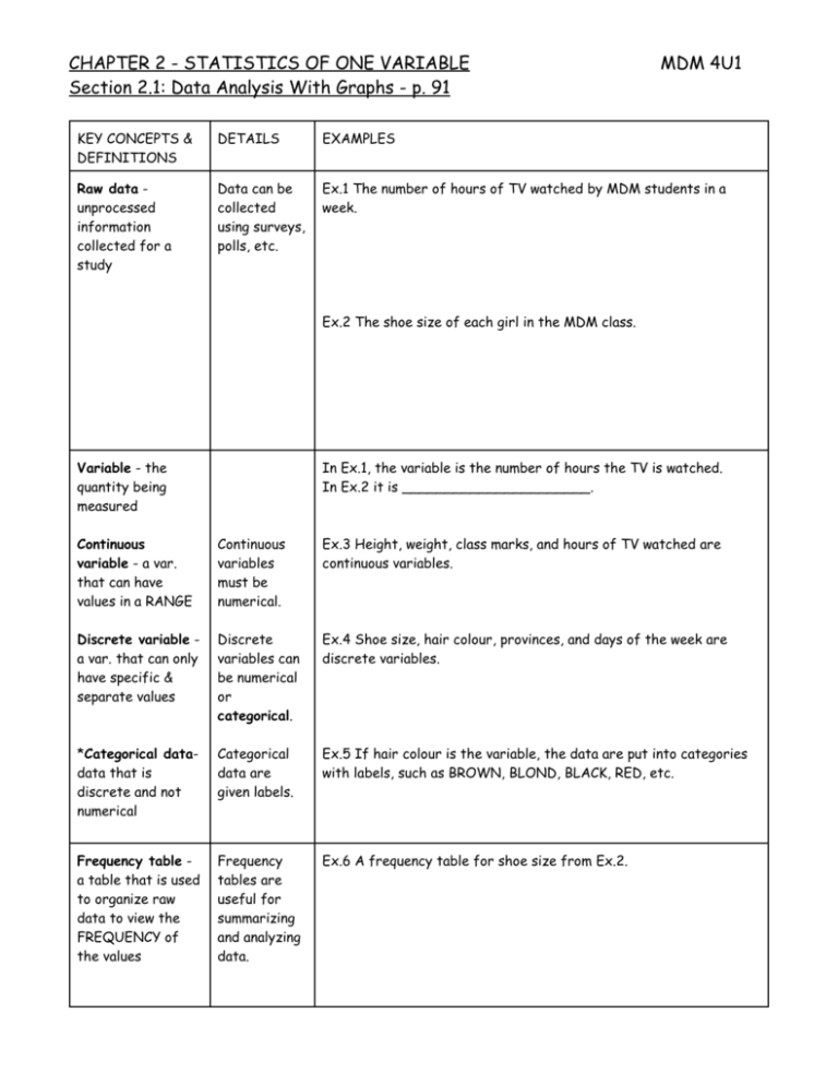
CHAPTER 2 - STATISTICS OF ONE VARIABLE
Section 2.1: Data Analysis With Graphs - p. 91
MDM 4U1
KEY CONCEPTS &
DEFINITIONS
DETAILS
EXAMPLES
Raw data unprocessed
information
collected for a
study
Data can be
collected
using surveys,
polls, etc.
Ex.1 The number of hours of TV watched by MDM students in a
week.
Ex.2 The shoe size of each girl in the MDM class.
Variable - the
quantity being
measured
In Ex.1, the variable is the number of hours the TV is watched.
In Ex.2 it is ______________________.
Continuous
variable - a var.
that can have
values in a RANGE
Continuous
variables
must be
numerical.
Ex.3 Height, weight, class marks, and hours of TV watched are
continuous variables.
Discrete variable a var. that can only
have specific &
separate values
Discrete
variables can
be numerical
or
categorical.
Ex.4 Shoe size, hair colour, provinces, and days of the week are
discrete variables.
*Categorical datadata that is
discrete and not
numerical
Categorical
data are
given labels.
Ex.5 If hair colour is the variable, the data are put into categories
with labels, such as BROWN, BLOND, BLACK, RED, etc.
Frequency table a table that is used
to organize raw
data to view the
FREQUENCY of
the values
Frequency
tables are
useful for
summarizing
and analyzing
data.
Ex.6 A frequency table for shoe size from Ex.2.
Frequency diagram
- a graph of the
data in a frequency
table
*Histogram - a
special type of bar
graph in which the
bars are connected
and represent a
continuous range
of values
(A regular bar
graph has bars
that are
separated,
indicating separate
categories)
For a large amount
of continuous data,
the data is usually
grouped into
classes or
intervals, which
makes the graphs
easier to construct
and interpret.
Typically, between
5 to 20 intervals
are used, that
must cover the
range of the data.
To find the range,
subtract the
smallest piece of
data from the
largest in the list.
A frequency
diagram could
be a
histogram, a
frequency
polygon (line
graph), a bar
graph, a pie
graph, or a
pictograph.
The first two
types of
graphs are
used most
often for
continuous
variables,
while the last
three are
used most
often for
discrete
variables.
Diagrams are
useful for
displaying and
analyzing
data.
Ex.7 A pie graph for shoe size from Ex.2.
Ex.8 A histogram for hours of TV watched from Ex.1.
Cumulative
frequency graph a graph that shows
the RUNNING
TOTAL of the
frequencies from
the lowest value up
(also called an
ogive)
Cumulative
freq. graphs
are good for
answering
questions
about the
data that
involve
proportion.
Ex.9 A cumulative frequency polygon for # of hours of TV watched.
What percentage of the students watch ____ hours of TV or less?
Relativefrequency graph a graph that shows
the frequency of a
data group as a
fraction of percent
of the whole data
set
Instead of
the y-axis
reading
“frequency”,
it will now
read “relative
frequency”
and be
expressed in
percent.
Ex.10 A relative-frequency graph for shoe size (bar graph).
HMK - p. 101 #1 (sol’ns wrong in txt), 2 (2c is vague), 3ab, 4ab, 5 (sol’n in txt has too many intervals), 7, 9
(error in txt with endpoints), 11, 13, 15
Section 2.3 - Sampling Techniques - p.113
When a STUDY or a SURVEY is done, it is often impossible/difficult to question
EVERYONE it concerns. Most often, researchers use a PERCENTAGE of people
concerned, called a SAMPLE.
POPULATION:
all individuals/items that belong to a group being studied.
SAMPLE:
a group of people/items SELECTED FROM a population.
*A sample must be chosen FAIRLY, as it is meant to REPRESENT the entire
population.
ex. Population - all students at Villy
Sample - our class
This would be a bad sample because it’s only grade 12 students, academic, etc.
A sample can be chosen in a number of fair ways. The choice of sampling techniques
depends on several factors - the nature of the population, cost, convenience, and
reliability, and is important for an accurate reflection of the population.
SAMPLING TECHNIQUES:
1.
SIMPLE RANDOM SAMPLE
When the population is made up of identifiable individuals who form one large group,
this technique is appropriate. Each member might be assigned a different number, and
then numbers can be randomly selected using a computer, out of a hat, etc.
ex. All men in Essex County over 50
2.
SYSTEMATIC SAMPLE
The pop’n is still made up of identifiable individuals who form one large group, but the
group may already be organized (ex. phone book, voter’s names, etc.). You select members
of the group at regular, sequential intervals (this is still random because you have no idea
who will be selected).
interval = population size / sample size
ex.
interval = 500 800 / 300 = 1670
choose ONE of the first 1670 members, and then every 1670th member on, in
every interval.
3.
STRATIFIED SAMPLE
When the pop’n is made up of DISTINCT GROUPS of members (the groups are called
STRATA), this sampling technique is used. It is used so that the SAMPLE has the same
PROPORTION of members from each stratum as the pop’n. You multiply the number of
members in each stratum by a desired percent.
ex. Salaries
# of members
sample (10% of the pop’n)
20000-40000
1200
0.10 x 1200 = 120
40001-60000
800
0.10 x 800 = 80
60001 or more
300
0.10 x 300 = 30
(2300 people)
(230 people)
4.
CLUSTER SAMPLE
When the pop’n is made up of GROUPS, but those groups are all very similar (and
likely to be representative of the entire pop’n), a number of groups are chosen randomly
for the sample.
ex. groups of employees at Roots stores across Canada
5.
MULTI-STAGE SAMPLE
This technique uses SEVERAL LEVELS of random sampling to narrow down the
sample.
ex. Population - all students in Ontario secondary schools
Sample - 1st, randomly select some municipalities
2nd, randomly select some schools WITHIN those municipalities
3rd, randomly select some students WITHIN those schools
6.
VOLUNTARY-RESPONSE SAMPLE (not as fair or representative as other methods)
This technique involves all members of the pop’n to participate VOLUNTARILY.
ex. call-in show
mail-in from a magazine
email response
survey posted on a bulletin board
7.
CONVENIENCE SAMPLE (not as fair or representative as other methods)
Sample groups are chosen for convenience and may not be representative).
ex. Population - all students at Villi
Sample - our class
HMK -
p.117 #1-4,6,8,11
Section 2.4 - Bias in Surveys - p.119
BIAS:
systematic error or undue weighting in a statistical study.
(Any factor that favours certain outcomes or responses and hence skews the study
results).
Bias can occur from choosing the wrong sample and/or collecting data incorrectly.
Bias is USUALLY unintentional, but is sometimes intentional to PURPOSELY skew results
to a more desirable outcome.
1.
SAMPLING BIAS
This occurs when the sample does not reflect the characteristics of the population.
ex. To conduct a survey about when the next school dance should be, students in
the library during all four periods are polled.
2.
NON-RESPONSE BIAS
This occurs when people who are surveyed refuse to participate. Those who are more
concerned may respond more readily, skewing the results.
3.
RESPONSE BIAS
This occurs when respondents DELIBERATELY give false or misleading answers in a
survey. Again, this may be done due to the wording of the questions that may
anger/embarass/etc. respondents.
4.
MEASUREMENT BIAS
This occurs when the method for collecting the data affects the variable it is
measuring consistently (under or overestimates the variable, which no longer represents
the population characteristic).
This could happen in one of three main ways.
The METHOD OF COLLECTION can be a problem (who collects the data or how it is
collected).
ex. Having a teacher survey the number of students who smoke on school property
(students may lie to teacher and so the measurement will be LOWERED and will
no longer be accurate).
If data is collected using QUESTIONS, it is very important how they are worded, or
they can produce also produce measurement bias.
LEADING QUESTIONS will lead an individual to choose an answer they might not
otherwise have chosen, thereby OVERESTIMATING the measurement, and skewing
results.
ex. What is your favourite colour?
a)
blue
b) green
c)
red
d) other __________
Since it is easier to choose a,b, or c, the results will likely be skewed.
LOADED QUESTIONS contain wording or information intended to influence the
respondent’s answer, thereby UNDER/OVERESTIMATING the measurement.
ex. Do you favour the new uniform policy which will ban flip flops?
(Should read: Do you think the new uniform policy is fair?)
HMK -
p.123 #1-6,8
Section 2.5 - Measures of Central Tendency - p.125
When data is collected, people often want to know the “average” of the data (often
for comparison purposes).
“Average” can be measured mathematically in three different ways, each with
advantages/disadvantages.
___________________________________________________________________
1.
MEAN: the sum of the values of a variable divided by the number of values.
POPULATION MEAN
SAMPLE MEAN
(often used to approximate the pop’n mean)
x + x 2 +...+ x µ= 1
∑x
µ=
µ:
_
x=
_
x=
x 1 + x 2 +...+ x n
n
∑x
n
mu (population mean)
_
x:
∑
x-bar (sample mean)
:
N:
n:
2.
MEDIAN:
3.
MODE:
sigma (the sum of)
the number of values in the population
the number of values in the sample
the middle value of the data when it is ranked from highest to lowest.
For an even number of data (and therefore 2 middle values), take the
mean of the tow middle values.
the value that occurs most frequently in a set of values. There may be no
mode, one mode, or several modes.
___________________________________________________________________
Some sets of data have OUTLIERS (values that are DISTANT from the MAJORITY
of the data).
In a small sample:
•
outliers can greatly affect the MEAN
•
the MEDIAN is less affected by outliers
•
the MODE may not exist or may an outlier!
•
mean, median, and mode may not agree
In a large sample (the more data, the better):
•
outliers have less effect on MEAN
•
MEDIAN is even more accurate
•
MODE is likely to be more accurate
•
mean, median, and mode are likely to be close
*WEIGHTED MEAN
A weighted mean must be used when all of the data is not equally as important.
Ex.1 Your marks on a quiz (with a weight of 4) vs. a test (with a weight of 8),
65% and 80%.
_
We cannot calculate mean with
both marks as equally important.
Instead, we use this formula:
w x + w 2 x 2 +...+ w n x n
xw = 1 1
w 1 + w 2 +...+ w n
x = (65 + 80) / 2 = 72.5, because that would count
_
_
wn :
or
xw =
∑w x
∑w
n
n
n
n
n
the weighting factor for the value x n
4( 65 ) + 8( 80 )
4+8
260 + 640
=
12
900
=
12
= 75%
_
x=
(counting 65 four times and 80 eight times)
*DATA GROUPED INTO INTERVALS
(Mode cannot be found because we don’t know how many times EACH value in the
INTERVAL occurs, we just have a total for the interval).
MEAN can be approximated using the midpoint value ( m n ) for each interval, and the
frequency ( f n ) for that interval.
∑f m
µ≈
∑f
(population)
∑f m
x≈
∑f
n
_
and
n
n
n
n
(sample)
MEDIAN can be approximated by taking the midpoint of the interval within which the
median is found (the midpoint is located by analyzing cumulative frequencies).
HMK -
p.132 #1-4,7,8,9 (9d should read bar graph, not histogram),11,14 (good
communication question, answer to 14b in text is incomplete)
Section 2.6: Measures of Spread - p. 136
Recall:
Measures of central tendency indicate the average or central values of a set of data.
NOW:
Measures of spread indicate how closely a set of data clusters around its centre.
The measure of spread discussed will depend on whether the MEAN or the MEDIAN has
been calculated. There is no measure of spread for the mode.
MEASURE OF SPREAD FOR THE MEAN:
The STANDARD DEVIATION and VARIANCE of a set of data show how the data cluster
around the mean of the data.
A Z-SCORE shows how FAR a datum (one data value) is from the mean, numerically, in terms
of standard deviations.
STANDARD DEVIATION:
Deviation - the difference between a value and the mean.
ex. 70% - 65% = 5% deviation
58% - 65% = -7% deviation
(mark) (mean)
(negative dev. b/c mark < mean)
The larger the deviations, the greater the SPREAD of the data.
Standard Deviation - the square root of the mean of the squares of the deviations.
*The “standard” deviation is like the “average” deviation for a data value.
*(see table and calculations on the next page)
(Sigma)
σ=
∑( x − µ )
2
N
(Pop’n)
s=
∑ (x − x )
n− 1
(Sample)
2
*there is greater weight on
larger deviations due to
the squaring
**A small standard deviation indicates that data cluster CLOSELY around the mean, while a
larger st. dev. indicates that the data is quite spread out.**
Ex. 1 Quiz scores (out of 10) for a class of 16 students. Calculate the stand. dev.
5
7
9
6
5
10
8
2
11
8
7
7
6
9
5
First, we must decide if we are using the pop’n or the sample formula. Because it’s the
whole class (not a sample), we will use the pop’n formula.
For the formula for σ , we need µ, x − µ, ( x − µ )
N is 16 (total number of data).
2
and N. We will make a table.
8
x−µ
Data
(x − µ)2
2
5,5,5
6,6
7,7,7
8,8,8
9,9
10
11
VARIANCE:
Variance - the mean of the squares of the deviations (the square of standard deviation!)
*(ACTUAL mathematical measure of spread vs. standard deviation, but more difficult to
understand because it is in SQUARE units; quality control use as an example of variance
application)
2
σ =
∑( x − µ )
2
N
(Pop’n)
2
s =
∑ (x − x)
n− 1
2
(Sample)
Ex. 2 Find the variance for the data in Ex. 1.
Z-SCORE (not a measure of spread)
A z-score is the number of standard deviations that a datum is from the mean.
z=
x−µ
(Pop’n)
σ
z=
x− x
s
(Sample)
*The z-score is found by dividing the deviation of the datum by the standard deviation.
Ex. 3 Determine the z-score of the marks 5/10 and 10/10 from Ex. 1.
MEASURE OF SPREAD FOR THE MEDIAN:
Data that has been listed in ascending/descending order can be divided into QUARTILES
(four equal groups of data, separated by key values) or PERCENTILES (100 equal groups or
intervals, separated by key values for each “percentile”).
For data divided into quartiles, the INTERQUARTILE RANGE and SEMI-INTERQUARTILE
RANGE show how data clusters around a median.
QUARTILES:
A quartile divides a set of ordered data into four equal groups. The three “dividing” points
are Q1 (1st quartile), Q2 (2nd quartile or median), and Q3 (3rd quartile).
*Q1 is the median of the lower half of the data, and Q3 is the median of the upper half.
The INTERQUARTILE RANGE is Q3-Q1 (the range of the data in the middle half of the set).
The larger the interquartile range, the larger the SPREAD of the central half of the data.
The SEMI-INTERQUARTILE RANGE is half the interquartile range (measuring the spread
in the middle of the interquartile range). This measure is not as useful as the interquartile
range.
Ex. 4 Determine the median, Q1, Q3, and the ranges for the data in Ex. 1.
First, the data must be placed in order:
2
5
5
5
6
6
7
7
7
8
8
8
9
9
10
11
Data is sometimes said to be “within a quartile”, which really means within a quarter divided
by the three quartiles.
Ex. 5 The score of 2 is in the 1st quartile (or lower quartile).
PERCENTILES:
A percentile divides the data into 100 equal intervals. Each percentile is labelled
P1, P2, P3, ... , P99. In general, we refer to the nth percentile as Pn.
We say that “n” percent of the data is less than or equal to Pn, and (100 - n) percent are
greater than Pn.
Ex. 6 Use the data below (final grades for a class) to answer the questions.
35
38
41
44
45
45
47
50
51
53
63
56
57
58
58
59
60
62
62
62
62
63
63
64
64
65
65
66
67
67
67
68
68
69
69
70
72
72
73
74
75
75
76
78
79
81
82
82
83
84
86
86
87
88
90
91
92
94
96
98
a)
What is the 70th percentile for this data?
b)
What is the 25th percentile for this data?
c)
What percentile corresponds to a grade of 81%?
d)
What percentile corresponds to a grade of 82%?
(60 pieces of data)
HMK - p. 148 #1, 2b, 3 (3c wrong in text), 4, 5 (sample, not pop’n, though vague in question), 6abd
(sample, not pop’n as it should be), 7ab, 10, 11, 14 (a-ii & c wrong in text)
REVIEW HMK - p. 151 #1, 2 (for 2a, use larger # of intervals b/c the range is so large), 3ac, 4a-d,
5, 6, 7, 9, 10, 11, 12abc, 14, 15, 16ac, 18a (a-ii wrong in text), 19, 20ab (use sample, not pop’n like
text),
p.154 #1, 2, 3ac, 4, 5, 7, 8, 9
CHAPTER 2 - FORMULAS
µ=
∑x
∑w
n
n
xn
∑f m
∑f
n
xw =
∑x
x=
µ≈
wn
∑f m
∑f
n
x≈
∑ ( x − µ)
n
σ=
n
2
n
n
s=
∑ ( x − x)
n− 1
∑ ( x − x)
s =
n−1
2
z=
x− x
s
2
∑ ( x − µ)
σ =
2
2
z=
x− µ
σ
2