HW #1 Solutions
Carbon Mass Problem: Assuming an average surface pressure of 1000 mb, an average
tropospheric temperature of 255 K, and a global CO2 mixing ratio of 385 ppm, what is
the current atmospheric Carbon reservoir (in units of kg m-2)? Compare your
approximation with Table 2.3 in W+H.
Surface pressure of 1000 mb can be used to estimate the mass of air over a column, p =
mg/A, yielding m/A = 10000 kg m-2. We want to know how much of this mass is carbon.
The ratio of CO2 molecules to air molecules is given by the mixing ratio of 385 ppm.
That CO2 is well mixed means that this value holds throughout the atmosphere. The ratio
of carbon mass to air mass is the mixing ratio times the carbon mass per CO2 molecule
(12 AMU) divided by the air mass per air molecule (29 AMU). 385 ppm x (12/29) =
1.6x10-4. This is the fraction of the 10000 kg m-2 column mass which is carbon.
Therefore the carbon column burden is 1.6 kg m-2. This agrees spot on with W+H.
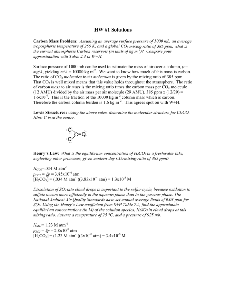
Lewis Structures: Using the above rules, determine the molecular structure for Cl2CO.
Hint: C is at the center.
Cl
Cl
C O
Henry’s Law: What is the equilibrium concentration of H2CO3 in a freshwater lake,
neglecting other processes, given modern-day CO2 mixing ratio of 385 ppm?
HCO2=.034 M atm-1
pCO2 = ξp = 3.85x10-4 atm
[H2CO3] = (.034 M atm-1)(3.85x10-4 atm) = 1.3x10-5 M
Dissolution of SO2 into cloud drops is important to the sulfur cycle, because oxidation to
sulfate occurs more efficiently in the aqueous phase than in the gaseous phase. The
National Ambient Air Quality Standards have set annual average limits of 0.03 ppm for
SO2. Using the Henry’s Law coefficient from S+P Table 7.2, find the approximate
equilibrium concentrations (in M) of the solution species, H2SO3 in cloud drops at this
mixing ratio. Assume a temperature of 25 °C, and a pressure of 925 mb.
HSO2= 1.23 M atm-1
pSO2 = ξp = 2.8x10-8 atm
[H2CO3] = (1.23 M atm-1)(3x10-8 atm) = 3.4x10-8 M
S+P problem 3.2:
This problem uses what we learned about termolecular reactions and applies it to the
conversion of NO2 to nitric acid via
NO2 + OH + M Æ HNO3 + M
Being a termolecular reaction, we know that this is the sum of three reactions, where we
have dropped the intermediary product HNO3* in the above reaction rate (see S+P). Thus
this “net” reaction doesn’t follow the Arrhenius form. Instead, the reaction rate is
obtained from Table B.2
R = k(T,z)[NO2][OH]
(1)
⎧
⎫ {1+[log10 ( k0 (T )[ M ] / k∞ (T )) ]2 }−1
k 0 (T )[M ]
k (T , z ) = ⎨
⎬0.6
+
k
T
k
T
1
(
(
)[
M
]
/
(
))
∞
0
⎩
⎭
−3
⎛ T ⎞
6
− 2 −1
k 0 (T ) = 2.0 x10 −30 ⎜
⎟ cm molecule s
⎝ 300 ⎠
−11
k ∞ (T ) = 2.5 x10 cm 3 molecule−1s −1
(2a,b,c)
Where k0(T)[M] is the rate for the low-pressure limit (i.e. damping collisions of HNO3*
with M are rare enough to be a limiting factor), and k∞(T) is the rate for the high pressure
limit (the rate of collisions between NO2 and OH is the limiting factor). You can see
from the form of (2a) that the slower rate dominates.
The concentration for the transition between low and high pressure limits, [M]t, is found
where k0(T)[M]t = k∞(T), this makes the denominator in (2a) = 2, and thus [M]t =
1.25x1019 molecules cm-3. Using p = [M]kT, we have pt = 0.52 atm. We take T = 300 K
for lack of guidance from the problem. Here I plot the solution with IDL.
S+P problem 3.4:
Collision theory predicts
RC = π (r1 + r2 ) v12 [OH][CHF3 ]
2
v12 =
8kT ⎛ 1
1 ⎞
⎜⎜
⎟
+
π ⎝ m1 m2 ⎟⎠
Plugging and chugging yields RC = 3.6x10-16 m3 molecule-1 s-1 [OH][CHF3]
= 3.6x10-10 cm3 molecule-1 s-1 [OH][CHF3]
Thus the fraction of collisions leading to a reaction, γ = k/3.6x10-10 = 7.7x10-7, or less
than one in a million. This is a rare reaction! First, the O side of OH has to hit the H side
of the HCF3. Furthermore, the collision has to be particularly energetic and “head on” so
the OH can “dig into” the electron shell and pull out the H atom without being deflected
first – note the relatively strong energy barrier (the exp(-E/T) term in k) seen in Table B.1
for this reaction (This was discussed in class on Monday. See S+P discussion in section
3.2.3 if you wonder what I’m talking about). Furthermore, the O side of OH is the more
negative side, and thus the electron shell around the fluorocarbon will be attracting the H
in the OH, further complicating the reaction
S+P Problem 3.6:
This problem deals with heterogeneous reaction (not discussed in class, but found in S+P
section 3.7). It follows directly from collision theory with three simplifications: 1) the
speed of the aerosol particle will be negligible compared to that of the gas molecule, so
v12 = vg; 2) the radius of the gas molecule will be negligible compared to that of the
aerosol, so d = ra; and 3) instead of an Arrhenius form for the reaction efficiency, we just
use a fixed fraction, γ. (Don’t get confused that S+P has a ¼ out front of (3.36). That’s
just because they use Ap = particle surface area, and have to put the ¼ out front to convert
back to cross-sectional area, which is more relevant for collision theory.)
Using these simplifications, we get
R = γRC = γπ (r1 + r2 ) v12 n A [ N 2 O 5 ]
2
= γπrA v g n A [ N 2 O 5 ]
2
vg =
8kT
πm
Where the term in front of the [N2O5] is the first order rate coefficient = 7.5x10-4 s-1. It
takes an N2O5 molecule about 20 minutes to find and react on the surface of an aerosol
particle…
S+P problem 3.8:
AÆBÆC
(1)
AÆB
BÆC
(1a)
(1b)
is equivalent to,
So the concentration equations are
d [ A]
= −k1a [ A]
dt
d [ B]
= k1a [ A] − k1b [ B]
dt
d [C ]
= k1b [ B]
dt
(2a,b,c)
a. part 1 -- Solve explicitly
(2a) is simple to solve,
[A] = [A]0exp(-k1at).
(3)
Using this in 2(b), we get
d[ B]
= k1a [ A]0 exp( − k1a t ) − k1b [ B ]
dt
(4)
Taking our lesson from the eigenvector/eigenvalue analysis, we’ll see that this problem
has solutions of the form.
[ B] = [ B] a exp(−k1a t ) + [ B]b exp(−k1b t )
Which yields
(4)
− [ B] a k1a exp(− k1a t ) − [ B]b k1b exp(− k1b t ) =
k1a [ A]0 exp(−k1a t ) − k1b ([ B] a exp(− k1a t ) + [ B]b exp(− k1b t ) )
Now we just group terms with the same eigenvalue (decay rate), and use the initial
condition that [B]0 = 0 to get
[ B]a =
k1a
[ A]
(k1b − k1a ) 0
[ B ]b = −[ B ] a
and
(5a,b)
[ B ] = [ A]0
k1a
(exp(−k1a t ) − exp(−k1bt ) )
(k1b − k1a )
(6)
Finally, we can solve for [C] by integrating (2c) with (6) and using the initial condition
that [C]0 = 0
[C ] = [ A]0
k1a k1b ⎛ [1 − exp(−k1a t )] [1 − exp(−k1b t )] ⎞
⎜
⎟⎟
−
(k1b − k1a ) ⎜⎝
k1a
k1b
⎠
(7)
You can check that this starts at zero and has a time derivative of zero at t=0, consistent
with the initial conditions for [C] that we imposed, and the fact that C’s source, which is
B, is also zero at t = 0. You can also see that as t >> 1/k1a + 1/k1b, then [C] Æ [A]0,
which is what we expect – that everything starting in A eventually ends up as C.
a. part 2 – justify PSSA for [B]
PSSA for [B] states that the source and sink terms for [B] are far larger than their
difference, d[B]/dt after some initial equilibrium reaction time. Using scale analysis on
(2b), we can formally express this condition as,
[ B]
<< k1a [ A] ~ k1b [ B ]
T
(8)
PSSA is concerned with the longer timescales of a set of reactions after a pseudo steady
state has been reached. If we set T to be the larger of 1/k1a or 1/k1b, then we get
[ B] <<
k1b [ B]
smaller of k1a , k1b
(9)
The only way for this to work is if k1a << k1b.
Here’s an alternate argument using the eigenvalue/eigenfunction analysis. PSSA is
justified when the two eigenvalues (i.e. adjustment rates) are well separated. In this case,
the eigenvalues are simply k1a and k1b (you can do the math). Plugging these in to solve
for the eigenvectors, we see that the k1a eigenvalue corresponds to an eigenvector where
[B] = [A]k1a/(k1b- k1a) and the k1b eigenvalue corresponds to a decay purely in [B].
If k1a >> k1b, we have a very boring solution that the rapid eigenvector points along the
[A]/[B] = -1 line, which simply means that [A] converts into [B] very rapidly through
(1a) until it reaches a state parallel to the second eigenvector, which points along [A] = 0.
You will note that this is the same as a PSSA problem where (2a) is set to zero. Since the
problem asked about setting (2b) to zero (not (2a)), we have to move on.
In the other case, where k1b.>> k1a, [B] quickly equilibrates (independently of [A]) until it
is on the line defined by the 1st eigenvector. The first eigenvector in this limit predicts
that [B]/[A] = k1a/k1b << 1. After reaching this pseudo-equilibrium, [A] and [B] decay
together towards zero at the slower rate k1a. This is a more meaningful use of PSSA, than
the k1b.>> k1a case, simply because there is some state where[A] and [B] are both nonzero and in pseudo-equilibrium.
b. Use PSSA to solve problem
Setting (2b) = 0 yields
[B] = [A]k1a/k1b
(10)
[A] = [A]0exp(-k1at).
(3)
[B] = [A]0(k1a/k1b)exp(-k1at)
(11)
The solution for (2a) is still (3).
Combining (3) and (10) yields
Integrating (2c) using (11) yields
[C] = [A]0[1-exp(-k1at)]
(12)
You could have also gotten (12) by noting that [A] + [B] + [C] = [A]0, and [B] << [A],
yielding [C] = [A]0 – [A]. You can easily reconcile (11) and (12) with (6) and (7) in the
limit that k1a << k1b.