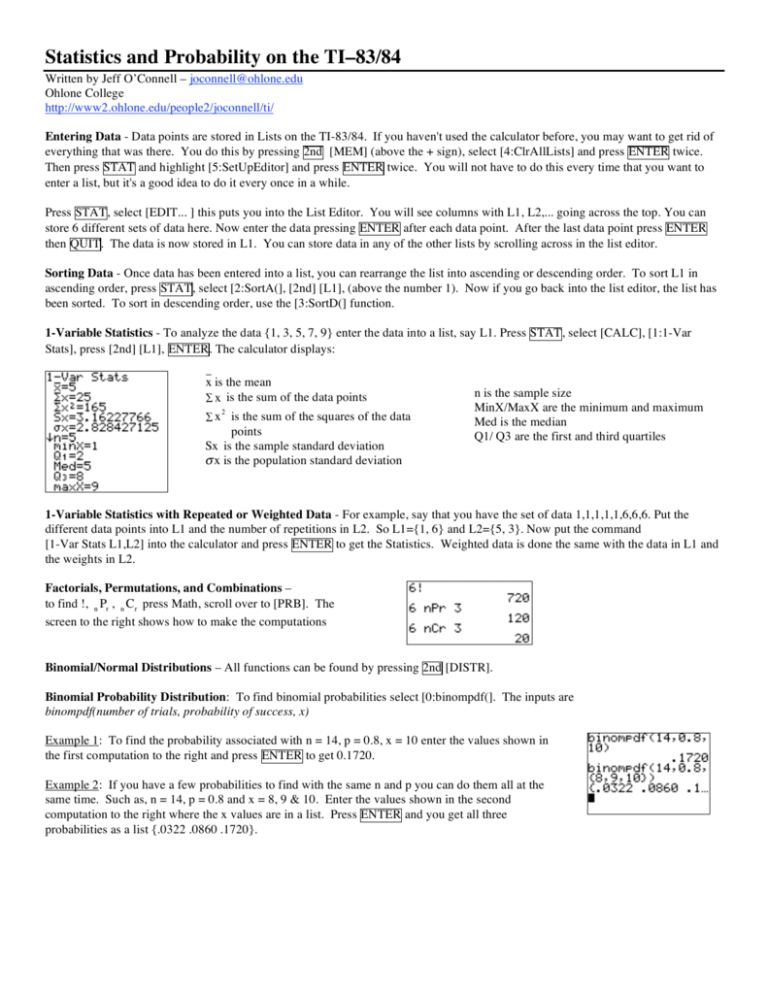
Statistics and Probability on the TI–83/84
Written by Jeff O’Connell – joconnell@ohlone.edu
Ohlone College
http://www2.ohlone.edu/people2/joconnell/ti/
Entering Data - Data points are stored in Lists on the TI-83/84. If you haven't used the calculator before, you may want to get rid of
everything that was there. You do this by pressing 2nd [MEM] (above the + sign), select [4:ClrAllLists] and press ENTER twice.
Then press STAT and highlight [5:SetUpEditor] and press ENTER twice. You will not have to do this every time that you want to
enter a list, but it's a good idea to do it every once in a while.
Press STAT, select [EDIT... ] this puts you into the List Editor. You will see columns with L1, L2,... going across the top. You can
store 6 different sets of data here. Now enter the data pressing ENTER after each data point. After the last data point press ENTER
then QUIT. The data is now stored in L1. You can store data in any of the other lists by scrolling across in the list editor.
Sorting Data - Once data has been entered into a list, you can rearrange the list into ascending or descending order. To sort L1 in
ascending order, press STAT, select [2:SortA(], [2nd] [L1], (above the number 1). Now if you go back into the list editor, the list has
been sorted. To sort in descending order, use the [3:SortD(] function.
1-Variable Statistics - To analyze the data {1, 3, 5, 7, 9} enter the data into a list, say L1. Press STAT, select [CALC], [1:1-Var
Stats], press [2nd] [L1], ENTER. The calculator displays:
x is the mean
! x is the sum of the data points
!x
2
is the sum of the squares of the data
points
Sx is the sample standard deviation
! x is the population standard deviation
n is the sample size
MinX/MaxX are the minimum and maximum
Med is the median
Q1/ Q3 are the first and third quartiles
1-Variable Statistics with Repeated or Weighted Data - For example, say that you have the set of data 1,1,1,1,1,6,6,6. Put the
different data points into L1 and the number of repetitions in L2. So L1={1, 6} and L2={5, 3}. Now put the command
[1-Var Stats L1,L2] into the calculator and press ENTER to get the Statistics. Weighted data is done the same with the data in L1 and
the weights in L2.
Factorials, Permutations, and Combinations –
to find !, n Pr , n Cr press Math, scroll over to [PRB]. The
screen to the right shows how to make the computations
Binomial/Normal Distributions – All functions can be found by pressing 2nd [DISTR].
Binomial Probability Distribution: To find binomial probabilities select [0:binompdf(]. The inputs are
binompdf(number of trials, probability of success, x)
Example 1: To find the probability associated with n = 14, p = 0.8, x = 10 enter the values shown in
the first computation to the right and press ENTER to get 0.1720.
Example 2: If you have a few probabilities to find with the same n and p you can do them all at the
same time. Such as, n = 14, p = 0.8 and x = 8, 9 & 10. Enter the values shown in the second
computation to the right where the x values are in a list. Press ENTER and you get all three
probabilities as a list {.0322 .0860 .1720}.
Binomial Cumulative Density Function: To find binomial cumulative probabilities select [A:binomcdf(]. The inputs are
binomcdf(number of trials, probability of success, x) and the result will be the sum of all probabilities less than or equal to x.
Example 3: To find the cumulative probability associated with n = 14, p = 0.8, x ! 10 enter the
values shown in the computation to the right and press ENTER to get 0.3018.
Normal Distributions: To find probabilities from the normal distribution select [2:normalcdf(]. The inputs are
normalcdf(lower bound, upper bound) if your dealing with the standard normal distribution or
normalcdf(lower bound, upper bound, µ, σ) if you are dealing with a normal distribution
Example 4: To find the area under the normal curve between z = –1.23 and z = 2.45 enter the
values shown in the first computation to the right and press ENTER to get 0.8835.
Example 5: To find the area under the curve between 17 and 24 of a normal distribution with
µ = 19 and σ = 2.5 enter the values shown in the second computation to the right and press ENTER
to get 0.7654.
Example 6: To find the area to the right of 24 of a normal distribution with µ = 19 and σ = 2.5 use
the fact that 1E99 is essentially +! as far as the computation is concerned and enter the values
shown in the third computation to the right and press ENTER to get 0.0228.
NOTE: Use –1E99 for !" .
Important note: You must keep in mind that the calculator is finding the area under the curve much more accurately than the z-table.
The z-table rounds the areas to 4 decimal places while the calculator rounds to 10 decimal places. This could cause your answers to
be slightly different than answers from the z-table. In the example 5 we got .7654 to 4 decimal places. If you used the z-table you
would get .7653. This is a minor difference but it is something that you need to keep in mind.