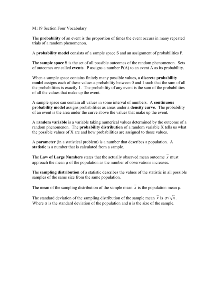
M119 Section Four Vocabulary
The probability of an event is the proportion of times the event occurs in many repeated
trials of a random phenomenon.
A probability model consists of a sample space S and an assignment of probabilities P.
The sample space S is the set of all possible outcomes of the random phenomenon. Sets
of outcomes are called events. P assigns a number P(A) to an event A as its probability.
When a sample space contains finitely many possible values, a discrete probability
model assigns each of these values a probability between 0 and 1 such that the sum of all
the probabilities is exactly 1. The probability of any event is the sum of the probabilities
of all the values that make up the event.
A sample space can contain all values in some interval of numbers. A continuous
probability model assigns probabilities as areas under a density curve. The probability
of an event is the area under the curve above the values that make up the event.
A random variable is a variable taking numerical values determined by the outcome of a
random phenomenon. The probability distribution of a random variable X tells us what
the possible values of X are and how probabilities are assigned to those values.
A parameter (in a statistical problem) is a number that describes a population. A
statistic is a number that is calculated from a sample.
The Law of Large Numbers states that the actually observed mean outcome x must
approach the mean  of the population as the number of observations increases.
The sampling distribution of a statistic describes the values of the 
statistic in all possible
samples of the same size from the same population.
The mean of the sampling distribution of the sample mean x is the population mean .
The standard deviation of the sampling distribution of the sample mean x is  / n .
Where  is the standard deviation of the population
 and n is the size of the sample.


Choose an SRS of size n from any population with mean  and finite standard deviation
. The Central Limit Theorem states that when n is large the sampling distribution of
x is approximately Normal. We can use the N(,  / n) distribution to approximate
probabilities involving x .
Events A and B are disjoint if they have no outcomes in common.


Events A and B are independent if knowing that one event occurred does not change the
probability we would assign to the other event.

For the Binomial Setting we have the following conditions:
1. There are a fixed number of observations.
2. The observations are independent.
3. Each observation has only one of two possibilities, typically called “success” and
“failure”.
4. The probability of “success” is the same for all observations. This probability is
typically called p.
If X has the binomial distribution with n observations and probability p of success on
each observation, the probability that X takes on any of the values 0, 1, 2, … n is
n 
P(X  k)   p k (1 p) nk
k 
The mean and standard deviation for the binomial count X are
 = np

  np(1 p)

The Normal approximation to the binomial distribution is N(np, np(1 p)) .
