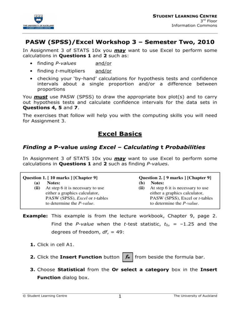
STUDENT LEARNING CENTRE
3rd Floor
Information Commons
PASW (SPSS)/Excel Workshop 3 – Semester Two, 2010
In Assignment 3 of STATS 10x you may want to use Excel to perform some
calculations in Questions 1 and 2 such as:
•
finding P-values
and/or
•
finding t-multipliers
and/or
•
checking your ‘by-hand’ calculations for hypothesis tests and confidence
intervals about a single proportion and/or a difference between
proportions
You must use PASW (SPSS) to draw the appropriate box plot(s) and to carry
out hypothesis tests and calculate confidence intervals for the data sets in
Questions 4, 5 and 7.
The exercises that follow will help you with the computing skills you will need
for Assignment 3.
Excel Basics
Finding a P-value using Excel – Calculating t Probabilities
In Assignment 3 of STATS 10x you may want to use Excel to perform some
calculations in Questions 1 and 2 such as finding P-values.
Question 1. [ 10 marks ] [Chapter 9]
(a) Notes:
(ii) At step 6 it is necessary to use
either a graphics calculator,
PASW (SPSS), Excel or t-tables
to determine the P-value.
Question 2. [ 9 marks ] [Chapter 9]
(b) Notes:
(ii) At step 6 it is necessary to use
either a graphics calculator,
PASW (SPSS), Excel or t-tables
to determine the P-value.
Example: This example is from the lecture workbook, Chapter 9, page 2.
Find the P-value when the t-test statistic, t0, = –1.25 and the
degrees of freedom, df, = 49:
1. Click in cell A1.
2. Click the Insert Function button
from beside the formula bar.
3. Choose Statistical from the Or select a category box in the Insert
Function dialog box.
© Student Learning Centre
1
The University of Auckland
STUDENT LEARNING CENTRE
3rd Floor
Information Commons
4. Choose TDIST from the Select a function box (Figure 1).
Figure 1
5. Click OK.
6. Fill the t-test statistic in the X dialog box.
Note: If your t-test statistic is negative, DON’T type the negative sign.
7. Type in the degrees of freedom (n – 1).
8. Enter 1 or 2 depending on whether the test is one-tailed or two-tailed
(Figure 2).
Figure 2
7. Click OK. (The value of 0.217237 should appear in cell A1.)
© Student Learning Centre
2
The University of Auckland
STUDENT LEARNING CENTRE
3rd Floor
Information Commons
Finding a t-multipler using Excel – Calculating the Inverse of
the Student t-distribution
In Assignment 3 of STATS 10x you may want to use Excel to perform some
calculations in Questions 1 and 2 such as finding t-multipliers.
Example: Find the t-multiplier for a 95% confidence interval with degrees
of freedom, df = 30. (That is: t30(0.025), probability 0.025 and 30 degrees
of freedom).
1. Click on cell A1.
2. Click the Insert Function button
from beside the formula bar.
3. Choose Statistical from the Or select a category box in the Insert
Function dialog box.
4. Choose TINV from the Select a function box (Figure 3).
Figure 3
5. Click OK
© Student Learning Centre
3
The University of Auckland
STUDENT LEARNING CENTRE
3rd Floor
Information Commons
6. Fill in the TINV dialog box (Figure 4).
Figure 4
Note:
The Excel function TINV calculates the t-value for a two–tailed t-distribution.
So if we want to find the t-value whose probability to the right is 0.1, then in
the TINV function the value for the probability is entered as 0.2, because of
the two-tailed nature of the function.
7. Click OK. (The value 2.042 should appear in cell A1.)
Note:
The examples can be solved by directly typing the formula =TINV(p, df) into
the cell, where:
p
is the probability for the two-tailed distribution
df
is the number of degrees of freedom for the distribution
© Student Learning Centre
4
The University of Auckland
STUDENT LEARNING CENTRE
3rd Floor
Information Commons
Downloading
Calculators
the
Excel
Test
and
Confidence
Interval
In Assignment 3 of STATS 10x you may want to use the Excel Test and
Confidence Interval Calculators to check your ‘by-hand’ calculations for
hypothesis tests and confidence intervals about a single proportion and/or a
difference between proportions in Question 1 and/or 2. These are available
to you in two places:
1. From Cecil (log in to Cecil in the usual way, click on Assignment
Resources and look for “Single/One proportion” and “Two
proportions”)
2. Go to Leila’s Student Learning
www.stat.auckland.ac.nz/~leila
Centre
STATS
10x
webpage
Question 2. [ 9 marks ] [Chapter 9]
(b) Notes:
(iii) You can check your calculations by using the Excel spreadsheet on Cecil. Look under
Assignment Resources.
Whichever way you do it, access Single/One proportion.xls and/or Two
proportions.xls now.
Let’s have a go at using these two documents!
On the following two pages are some questions from the Worked Examples
document which you can find on Cecil.
We won’t be doing the calculations by hand, although you are welcome to try
later – in this workshop we’ll use Excel to do them!
Question 13
[Chapter 9]
(similar to Question 2, Assignment 3)
In 2001, the New Zealand Planning Institute (NZPI) conducted a random
survey of its members. The NZPI survey included questions about job title,
location and the types of organisations members worked for. 324 responses to
these questions were received. Some of the information collected from the
responses were:
– 78 responses were received from Senior Planners.
– 38 responses were received from Managers.
– 116 members were located in Auckland.
– 83 members were located in Wellington/Christchurch.
– Of those members who were located in Auckland, 68 were planners
working for a Council.
– Of those members who were located in Wellington/Christchurch, 38
were planners working for a Council.
© Student Learning Centre
5
The University of Auckland
STUDENT LEARNING CENTRE
3rd Floor
Information Commons
(a)
State the sampling situation for the difference between the proportion of
NZPI senior planners and the proportion of NZPI members who are
located in Auckland.
(b)
By hand, test to see if there is a difference between the proportion of
NZPI members who are senior planners and the proportion who are
managers. Interpret your results.
1.
Parameter = pS – pM, the difference in the true proportion of NZPI
2.
members who are senior planners and the true proportion who are
managers.
H0: pS – pM = 0
3.
4.
H1: pS – pM ≠ 0
ˆS - p
ˆM , the difference in the proportion of the sample that
Estimate p
were senior planners and the proportion of the sample that
were managers.
78
38
=
= 0.2407 - 0.1173 = 0.1234
324 324
5.
Sampling situation (b): One sample of size n, several response
categories.
ˆS - p
ˆM ) =
se(p
t0 =
0.2407 + 0.1173 - 0.12342
= 0.032526
324
0.1234 - 0
= 3.794 ,
0.032526
df = ∞ (working with proportions)
6.
P-value = pr(T∞ > 3.794) + pr(T∞ < -3.794) = 2 x pr(T∞ > 3.794) =
0.0001 (from Excel)
7.
We have very strong evidence:
- against H0 in favour of H1.
- that the proportion of senior planners is not the same as the
proportion of managers.
The observed difference, 0.1234, is a statistically significant result at
the 5% level.
8.
Use estimate ± t x se(estimate), estimate = 0.1234, se(estimate) =
0.032526, t = z = 1.96
95% confidence interval is:
0.1234 ± 1.96 × 0.032526
= (0.0596, 0.1872)
9 With 95% confidence, we estimate that the proportion of NZPI members
who are senior planners is greater than the proportion who are
managers by between 0.06 and 0.19.
© Student Learning Centre
6
The University of Auckland
STUDENT LEARNING CENTRE
3rd Floor
Information Commons
Useful places to look for help by assignment question
Assignment
question
number
Worked
Examples
question
number
Lecture
Workbook
page
number
Q1
Q2
Q3
Q4
Q5
Q6
Q7
Also, don’t forget where else you can get assignment help! They are:
•
The STATS 10x forum: www.stat.auckland.ac.nz/forum/10x
•
Statistics Assistance Area – ask a tutor or your neighbour
•
Statistics Computer Lab – ask a lab demonstrator or your neighbour
•
Your lecturer’s office hours! See Cecil for details – if they don’t suit
you, email or call them to book a time.
© Student Learning Centre
7
The University of Auckland
STUDENT LEARNING CENTRE
3rd Floor
Information Commons
PASW (SPSS)
In Assignment 3 of STATS 10x you must use PASW (SPSS) to draw the
appropriate box plot(s) and to carry out hypothesis tests and calculate
confidence intervals for the data sets in Questions 4, 5 and 7. Instructions
on the question sheet read:
Hypothesis tests in this assignment
• In questions 4 and 5:
• You must follow steps 1, 2, 3, 7 and 9 in the “Step-by-Step Guide to Performing a t-test
by Hand”, Lecture Workbook, page 9, Chapter 9.
• Replace steps 4 – 6 and 8 in the “Step-by-Step Guide to Performing a t-test by Hand”
with the relevant computer output.
Computer use in this assignment
• Make sure you are prepared for questions 4, 5 and 7 before you begin to use the computer.
• Hand in computer output for questions 4, 5 and 7.
• Report P-values to 3 or 4 decimal places.
• When carrying out a two independent sample t-test using PASW (SPSS) do not assume
equal variances.
To save you typing time, all of the data files required for this workshop can be
found on Leila’s SLC STATS 10x website www.stat.auckland.ac.nz/~leila and
also on Cecil in PASW (SPSS) data file (.sav) format.
Paired Data Comparisons – finding the differences,
plotting the data and carrying out a paired t-test for the
mean difference and/or a sign test for the median
difference
Paired t-test
What is the correct null
hypothesis for this test?
Example: Conduct a paired data t-test for a mean difference of 0.
The head diameters of 18 N.Z. Airforce recruits were measured
twice, once using cheap cardboard calipers and again using
expensive and uncomfortable metal calipers.
© Student Learning Centre
8
The University of Auckland
STUDENT LEARNING CENTRE
3rd Floor
Information Commons
1.
Firstly, enter the data into PASW (SPSS) or open the Calipers.sav file.
2.
Secondly find the differences by:
a. Choose the Compute Variable tool:
Click Transform → Compute Variable
© Student Learning Centre
9
The University of Auckland
STUDENT LEARNING CENTRE
3rd Floor
Information Commons
b. Get the Compute Variable tool to find the differences:
i. Type “differences” into the Target Variable field.
ii. Click Cardboard.
iii. Click
.
iv. Click
(the subtraction button).
v. Click Metal.
vi. Click
.
vii. Click OK.
c. The differences will be computed and displayed in the Data Editor.
© Student Learning Centre
10
The University of Auckland
STUDENT LEARNING CENTRE
3rd Floor
Information Commons
3.
Thirdly, plot the differences using a boxplot.
a. Choose the Explore tool:
Click Analyze → Descriptive Statistics → Explore
b. Click on differences and then click on
to send it to the
Dependent List.
Click on Plots (at the bottom) so Statistics aren’t displayed.
Click on Plots (at the right) and deselect Stem-and-leaf so only a
boxplot is displayed. Click Continue.
© Student Learning Centre
11
The University of Auckland
STUDENT LEARNING CENTRE
3rd Floor
Information Commons
c. Click OK. The boxplot will appear in the Output window.
4.
Fourthly, carry out the paired t-test.
a. Choose the analysis tool: Paired-Samples T Test.
Click Analyze → Compare Means → Paired-Samples T Test.
© Student Learning Centre
12
The University of Auckland
STUDENT LEARNING CENTRE
3rd Floor
Information Commons
b. Select the variables of interest.
i. Cardboard is highlighted. Click
.
ii. Click on Metal.
iii. Click
.
iv. Click OK.
© Student Learning Centre
13
The University of Auckland
STUDENT LEARNING CENTRE
3rd Floor
Information Commons
5.
Lastly, view and interpret the results.
© Student Learning Centre
14
The University of Auckland
STUDENT LEARNING CENTRE
3rd Floor
Information Commons
The Sign Test
What is the correct null
hypothesis for this test?
Example: Conduct a sign test for a median difference of 0.
A study was designed to determine the effectiveness of a new diet.
Nine people took part in the study. The weight of each person was
recorded and then after three months on the diet, their weights
were again recorded.
1. Enter the data into PASW (SPSS) or open the Diet.sav file.
2. Choose the analysis tool: 2 Related Sample Nonparametric Test.
Click Analyze → Nonparametric Tests → Legacy Dialogs → 2
Related Samples.
© Student Learning Centre
15
The University of Auckland
STUDENT LEARNING CENTRE
3rd Floor
Information Commons
3. Select the relevant variables.
Click Before and After.
Click
.
4. Choose the test type(s).
Click the Wilcoxon box to unselect it. Click the Sign box.
Click OK.
5. View and interpret the results.
© Student Learning Centre
16
The University of Auckland
STUDENT LEARNING CENTRE
3rd Floor
Information Commons
Two Independent Samples – plotting the data
and carrying out a two independent samples t-test
What is the
correct null
hypothesis
for this test?
Example: Conduct a two independent
samples t-test for no difference in the means.
A random sample of 40 cellphones of the same make and model were chosen.
Half of the cellphones were randomly selected to have a nickel-cadmium
battery put in them and the rest had a nickel-metal hydride battery. The talk
time (in minutes) before the batteries needed to be recharged was recorded.
1.
Enter the data into PASW (SPSS) or open the Batteries.sav file.
Use a value of 1 for Nickel-cadmium and 2 for Nickel-metal
hydride.
2.
Assign labels.
Label the values:
Label 1 as Cadmium and 2 as Metal.
© Student Learning Centre
17
The University of Auckland
STUDENT LEARNING CENTRE
3rd Floor
Information Commons
3.
Plot the data using a boxplot.
a. Choose the Explore tool:
Click Analyze → Descriptive Statistics → Explore
b. Assign the variables.
Quantitative (response) variable → Variable box.
Click Time.
Click
.
Qualitative variable (grouping factor) → Category Axis box.
Click Battery.
Click
.
© Student Learning Centre
18
The University of Auckland
STUDENT LEARNING CENTRE
3rd Floor
Information Commons
c. View and interpret the boxplots.
4.
Carry out the two independent sample t-test.
a. Choose the analysis tool: Independent-Samples T Test.
Click Analyze → Compare Means → Independent-Samples T
Test.
© Student Learning Centre
19
The University of Auckland
STUDENT LEARNING CENTRE
3rd Floor
Information Commons
b. Select the variables of interest.
Quantitative variable (response) →
Test Variable(s) box.
Click Time.
Click top
.
Qualitative variable (grouping
factor) → Grouping Variable box.
Click Battery.
Click bottom
.
c. Define the direction of the difference (mean 1 – mean 2 or mean 2
– mean 1).
Click Define Groups.
Type 1 in the Group 1 box and type 2 in the Group 2 box.
Click Continue and then OK.
d. View and interpret the results.
© Student Learning Centre
20
The University of Auckland
STUDENT LEARNING CENTRE
3rd Floor
Information Commons
F-test for one-way ANOVA
What is the correct null
hypothesis for this test?
Example: Conduct a one-way ANOVA F-test for no difference in the groups’
underlying means.
Fifty students learned about the reading methods of ‘mapping’ and
‘scanning’. The method used and increase in reading age was
recorded for each student.
1.
Enter the data into SPSS or open the ReadingMethods.sav file.
Use a value of 1 for MapOnly, 2 for MapScan, 3 for Neither, and 4
for ScanOnly for the Method variable (Values column in the
Variable View).
Label Score as Increase in reading age and Method as Reading
Method.
2.
Plot the data using a boxplot.
a. Choose the Boxplot tool:
Click Graphs → Legacy Dialogs → Boxplot
© Student Learning Centre
21
The University of Auckland
STUDENT LEARNING CENTRE
3rd Floor
Information Commons
b. Pick the appropriate
plot.
c. Assign the variables.
Simple is
selected
by default.
Click
Define.
Quantitative (response)
variable → Variable box.
Click Increase in Reading
Age [increase].
Click
.
Qualitative variable (grouping
factor) → Category Axis box.
Click Reading Method
[method].
Click
.
Click OK.
d. View and interpret the boxplots.
© Student Learning Centre
22
The University of Auckland
STUDENT LEARNING CENTRE
3rd Floor
Information Commons
5.
Carry out the F-test.
a. Select the analysis tool: One-Way ANOVA.
Click Analyze → Compare Means → One-Way ANOVA.
b. Select the relevant variables.
Quantitative (response) variable → Dependent List box.
Click Increase in Reading Age [Score].
Click
.
Qualitative variable (grouping factor) → Factor box.
Click Reading Method [Method].
Click
.
3.
Select the relevant output tables.
Click Post Hoc.
Click the Tukey box.
Click Continue.
© Student Learning Centre
23
The University of Auckland
STUDENT LEARNING CENTRE
3rd Floor
Information Commons
Click Options.
4.
Click the Descriptive box.
Click Continue and then click OK.
View and interpret the results.
© Student Learning Centre
24
The University of Auckland