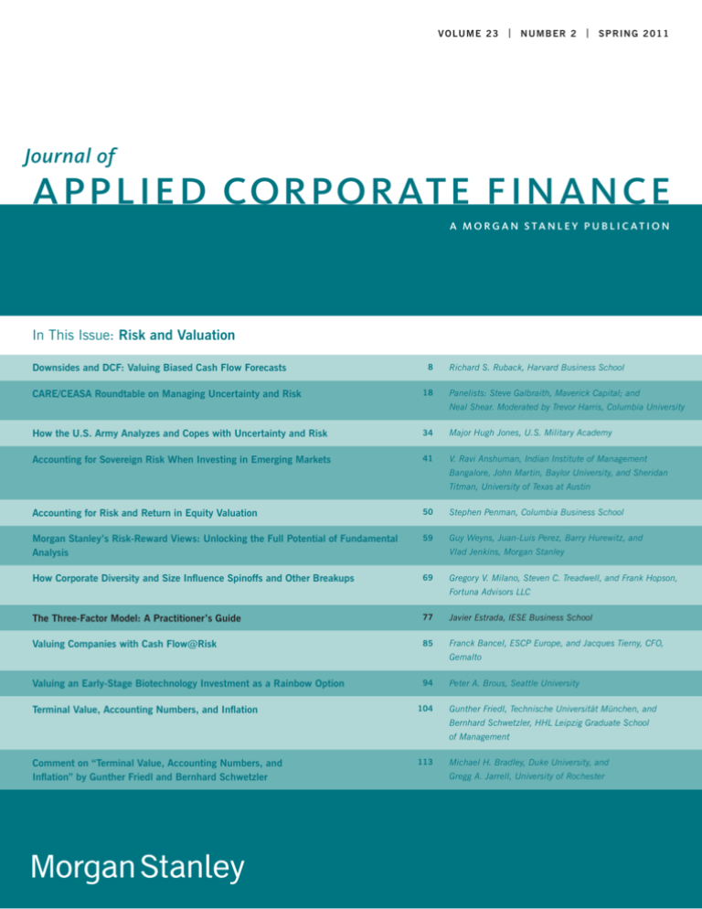
V O LU M E 2 3 | N U M B E R 2 | S P R IN G 2 0 1 1
Journal of
APPLIED CORPORATE FINANCE
A MO RG A N S TA N L E Y P U B L I C AT I O N
In This Issue: Risk and Valuation
Downsides and DCF: Valuing Biased Cash Flow Forecasts
CARE/CEASA Roundtable on Managing Uncertainty and Risk
8
18
Richard S. Ruback, Harvard Business School
Panelists: Steve Galbraith, Maverick Capital; and
Neal Shear. Moderated by Trevor Harris, Columbia University
How the U.S. Army Analyzes and Copes with Uncertainty and Risk
34
Major Hugh Jones, U.S. Military Academy
Accounting for Sovereign Risk When Investing in Emerging Markets
41
V. Ravi Anshuman, Indian Institute of Management
Bangalore, John Martin, Baylor University, and Sheridan
Titman, University of Texas at Austin
Accounting for Risk and Return in Equity Valuation
50
Stephen Penman, Columbia Business School
Morgan Stanley’s Risk-Reward Views: Unlocking the Full Potential of Fundamental
Analysis
59
Guy Weyns, Juan-Luis Perez, Barry Hurewitz, and
How Corporate Diversity and Size Influence Spinoffs and Other Breakups
69
Vlad Jenkins, Morgan Stanley
Gregory V. Milano, Steven C. Treadwell, and Frank Hopson,
Fortuna Advisors LLC
The Three-Factor Model: A Practitioner’s Guide
77
Javier Estrada, IESE Business School
Valuing Companies with Cash Flow@Risk
85
Franck Bancel, ESCP Europe, and Jacques Tierny, CFO,
Gemalto
Valuing an Early-Stage Biotechnology Investment as a Rainbow Option
Terminal Value, Accounting Numbers, and Inflation
94
104
Peter A. Brous, Seattle University
Gunther Friedl, Technische Universität München, and
Bernhard Schwetzler, HHL Leipzig Graduate School
of Management
Comment on “Terminal Value, Accounting Numbers, and
Inflation” by Gunther Friedl and Bernhard Schwetzler
113
Michael H. Bradley, Duke University, and
Gregg A. Jarrell, University of Rochester
The Three-Factor Model: A Practitioner’s Guide
by Javier Estrada, IESE Business School*
here is no doubt that the Capital Asset Pricing
Model (CAPM) is one of the models most widely
used in finance.1 But despite its widespread use,
the CAPM is far from uncontroversial. Debate
on its merits has been raging on for decades, and a consensus
on its usefulness is nowhere in sight.
That being said, of the many models that have challenged
the supremacy of the CAPM over the years, only one has slowly
but steadily emerged to become a strong contender—namely,
the three-factor model (3FM). This model aims to assess risk
more comprehensively than the CAPM, and thereby provide
a more reliable estimation of an asset’s required return. That
required return can be used as an input in the calculation of
the cost of capital, an important variable in most corporate
investment decisions, and also as an input in the calculation
of excess returns, a measure at the center of performance
evaluation and portfolio management.
This article aims to provide practitioners with a practical introduction to the 3FM by discussing an alternative to
the CAPM for estimating required or expected returns. To
that end, it discusses the model’s foundations, intuition, and
applications to both corporate finance and portfolio management.
T
premium should be estimated as the product of the market
risk premium and the asset’s beta. The market risk premium
is the compensation required by investors for investing in
relatively risky stocks as opposed to (ultimately risk-free)
government bonds. Beta is a measure of the sensitivity of
the asset’s returns to fluctuations in the market’s returns;
assets with a beta higher (lower) than 1 magnify (mitigate)
the market’s fluctuations. According to the CAPM, then, the
risk premium of asset i can be estimated as follows:
RPi = MRP∙βi
(2)
where MRP represents the market risk premium and βi is
the beta of asset i. As noted earlier, and is also apparent from
expression (2), the market risk premium is the same for all
assets, whereas beta is specific to the asset considered.
Combining equations (1) and (2) we get the following:
R i = R f + MRP∙βi ,
(3)
The risk-free rate is the compensation required for the
expected loss of purchasing power, and the risk premium is
the compensation for bearing the risk of an asset. As expression (1) shows, the risk-free rate is the same for all assets,
whereas the risk premium is specific to the asset considered.
This risk premium is precisely what the CAPM provides a
way to estimate. In fact, this model suggests that an asset’s risk
which is the usual way to express the CAPM. Note that this
expression yields both the required return and the expected
return for a given asset. This is the case because, in the equilibrium assumed by this model, whenever these two returns
are different, prices are assumed to adjust to restore the equality. For example, if investors require a 10% annual return
from an asset but expect it to yield 15%, buying pressure is
expected to drive the asset’s price up and its expected return
down. Conversely, if investors expect this asset to yield only
5%, selling pressure is expected to push the asset’s price down
and its expected return up. In both cases, the adjustment is
expected to continue until the required and the expected
return are the same.
The intuition behind expression (3) is straightforward.
The CAPM suggests that investors should require compensation for the expected loss of purchasing power and for bearing
risk. And it specifies that the compensation for risk should
be measured by the risk premium required for investing in
* This article draws heavily from Chapter 8 of my book The FT Guide to Understanding Finance, FT Prentice Hall, 2011. I would like to thank Mark Kritzman and Jack
Rader for their comments. Gabriela Giannattasio provided valuable research assistance.
The views expressed below and any errors that may remain are entirely my own.
1. Over 70-80% of practitioners claim to use this model to estimate the cost of eq-
uity; see Robert Bruner, Kenneth Eades, Robert Harris, and Robert Higgins (1998), “Best
Practices in Estimating the Cost of Capital: Survey and Synthesis,” Financial Practice
and Education, Spring/Summer, 13-28, and John Graham and Campbell Harvey (2001),
“The Theory and Practice of Corporate Finance: Evidence from the Field,” Journal of
Financial Economics, 60, 187-243.
A Brief Review of the CAPM
The required return on any asset i (R i ) can be estimated as
the sum of two variables: the risk free rate (R f ) and the asset’s
risk premium (RPi ). Expressed as an equation,
R i = R f + RPi .
Journal of Applied Corporate Finance • Volume 23 Number 2
(1)
A Morgan Stanley Publication • Spring 2011
77
relatively risky stocks instead of less risky bonds, adjusted by
a factor specific to each asset that reflects how much more or
less risky the asset is relative to the market.
The simplicity of this model, however, conceals a very
strong statement. Recall that beta is a measure of systematic risk. That implies that bankruptcy risk, liquidity risk,
currency risk, and as many others sources of firm-specific
or “idiosyncratic” risk as you can imagine are all irrelevant
when assessing the required return of an asset (though some
of these factors may be reflected in beta and therefore have
a systematic component). Liquidity, as the recent financial
crisis reminded us, is a good example of a risk that seemed to
pervade the entire financial system.
And yet, however strong this statement may be, a
supporter of the CAPM would justify it in at least two ways.
The first argument would be theoretical; it would claim
that, unlike the vast majority of its contenders, the CAPM is
solidly grounded in theory. In fact, it would argue that in a
world in which investors behave optimally, beta must be the
only relevant risk factor. In other words, the CAPM’s strong
statement is not an assumption but the result of a model of
optimal behavior.
The second argument would be empirical; it would
claim that a vast amount of research supports the plausibility of the CAPM. But this is a tricky argument. There is a
massive amount of research testing the validity of the CAPM
in different countries, over different time periods, and with
different methodologies. The problem is that there is a huge
amount of evidence on both sides of the fence. Those who
support the CAPM and those who dismiss it can point to a
vast amount of evidence that supports their position. As a
result, the evidence alone does not enable to either embrace
or reject the CAPM.
The Size and Value Premiums
And yet at least some empirical evidence is surprisingly
consistent. Data for different countries and over different
time periods show a consistent negative relationship between
market capitalization and returns; that is, over the long term,
small companies tend to deliver higher returns than large
companies. This empirical regularity is usually known as the
size premium.2
Similarly, data for different countries and over different
time periods show a consistent positive relationship between
book-to-market ratios (BtM) and returns; in the long term,
companies with high BtM tend to deliver higher returns
than those with low BtM. Recall that this ratio is a measure
of cheapness in the sense that high and low BtM indicate
cheap and expensive stocks relative to book value. And the
evidence shows that, over the long run, cheap (also known
as “value”) stocks tend to outperform expensive (also called
“growth”) stocks. This empirical regularity is usually known
as the value premium.3
But if the evidence on the size and value premiums is
rather clear, the theoretical reasons for the existence of these
premiums are much less convincing. In other words, no model
of optimal behavior leads to a result in which stock returns
depend on market cap and BtM. Some may not consider this
a problem; they would claim that, as long as we can isolate
the variables that explain differences in returns, we should use
them to determine required or expected returns. Yet others
would argue that there is no point using models that do not
follow from a sound underlying theory. You can pick your
side on this debate.
If you think a bit about it, though, these two risk premiums seem to make sense. Small companies are likely to be
less diversified and less able to survive negative shocks than
large companies. As for cheap companies, well, there must
be a reason why they are cheap! When buying value stocks,
investors are expecting a rebound but may get a falling knife.
In short, it is not hard to come up with plausible stories to
explain why small and cheap stocks are riskier than large
and expensive stocks, and therefore why they should deliver
higher returns.
But those are just stories. A better alternative may be
to establish empirical links from size and value to credible
sources of risk. The evidence on this seems to point to the fact
that small companies and value companies are less profitable
(they have lower earnings or cash flow relative to book value)
than large companies and growth companies. In other words,
small companies and value companies may be distressed
because of their poor profitability, and are therefore perceived
by investors as riskier.4
To summarize, then, the CAPM suggests that stocks with
high systematic (or market) risk should outperform those with
low systematic risk. In addition, the evidence quite clearly
shows that small stocks outperform large stocks; that cheap
(value) stocks outperform expensive (growth) stocks; and that
small and value companies are less profitable than large and
growth companies. Putting all this together, we conclude
that stock returns are determined by a market premium, a
size premium, and a value premium—and that is the main
insight of the 3FM.
One last issue before we discuss this model. Although
the evidence on the existence of the size and value premiums is largely undisputed, there is a heated controversy about
2. One of the earliest analysis of the relationship between size and stock returns is in
Rolf Banz (1981), “The Relationship Between Return and Market Value of Common
Stocks,” Journal of Financial Economics, 9, 3-18.
3. Although value investing has a very long history, one of the earliest formal analysis
of the relationship between cheapness and stock returns is in Sanjoy Basu (1983), “The
Relationship Between Earnings Yield, Market Value, and Return for NYSE Common
Stocks: Further Evidence,” Journal of Financial Economics, 12, 129-156.
4. See Cliff Asness, John Liew, and Ross Stevens (1997), “Parallels Between the
Cross-Sectional Predictability of Stock and Country Returns,” Journal of Portfolio Management, Spring, 79-87.
78
Journal of Applied Corporate Finance • Volume 23 Number 2
A Morgan Stanley Publication • Spring 2011
whether or not the excess returns of small and value stocks
(relative to large and growth stocks) are the result of their
higher risk. Some argue that this is not the case; that is, small
and value stocks are not riskier than large and growth stocks,
and therefore the additional returns they provide are a free
lunch courtesy of an inefficient market. Yet others argue
exactly the opposite; that is, small and value stocks offer
higher returns than large and growth stocks precisely because
they are riskier, which is exactly what one would expect in
an efficient market.
Again you can pick your side on this debate, but it’s
important to keep in mind that estimating required returns
with the 3FM amounts to an implicit acceptance of the
second point of view. This is the case because, as we will
discuss shortly, this model states that the higher an asset’s
exposure to the size and value premiums—in other words,
the higher the asset’s risk as defined by the 3FM—the higher
should be the asset’s required return.
An Overview of the 3FM
Estimating required returns with the 3FM is just a bit more
difficult than with the CAPM because we need to estimate
two more risk premiums and two more betas, for which we
need some additional data. Other than that, the model poses
no real challenge for any practitioner that wants to implement it.
According to the 3FM, the required return on an asset
follows from its exposure to the market, its size (measured
by market cap), and its valuation (measured by BtM). More
precisely, the required return on any asset i follows from the
expression
R i = R f + MRP∙βi + SMB∙βiS + HML∙βiV ,
(4)
where SMB (small minus big, referring to market cap) and
HML (high minus low, referring to BtM) denote the size
premium and the value premiums, and βiS and βiV denote the
return sensitivity of asset i to changes in these premiums.
Let’s think a bit about this expression. Recall that the
market risk premium (MRP) seeks to capture the additional
compensation required by investors for investing in relatively
riskier stocks as opposed to relatively safer bonds. Recall
also that it is measured by the average historical difference
between the return of a widely diversified portfolio of stocks
and the return of government bonds. And recall, finally, that
βi measures the sensitivity of asset i’s risk premium (RPi = R i
–R f ) to fluctuations in the market risk premium.
In similar fashion, the size premium (SMB) seeks to
capture the additional compensation required by investors for
investing in relatively riskier small companies as opposed to
5. Their seminal article on the subject is Eugene Fama and Kenneth French (1992),
“The Cross-Section of Expected Stock Returns,” Journal of Finance, 47, 427-465.
Journal of Applied Corporate Finance • Volume 23 Number 2
relatively safer large companies. The size premium is measured
by the average historical difference between the returns of a
portfolio of small stocks and those of a portfolio of large
stocks. And the beta associated with this factor, usually called
the size beta (βiS ), measures the sensitivity of asset i’s risk
premium to fluctuations in the size premium.
Finally, the value premium (HML) seeks to capture the
additional compensation required by investors for investing in relatively riskier value stocks as opposed to relatively
safer growth stocks. The value premium is measured by the
average historical difference between the returns of a portfolio of high-BtM stocks and those of a portfolio of low-BtM
stocks. And the beta associated with this factor, usually called
the value beta (βiV ), measures the sensitivity of asset i’s risk
premium to fluctuations in the value premium.
Note that, just as we stressed earlier about the MRP,
neither SMB nor HML in expression (4) have a subscript i.
This means that the size and value premiums (as well as the
risk-free rate and the market risk premium) are the same for
all assets. Conversely, note that the size beta and the value
beta (as well as the market beta) do have a subscript i, and
therefore are specific to the asset considered.
Implementation of the 3FM
Like the CAPM, the 3FM is silent about several practical
issues that are inevitably faced when implementing this model.
What is an appropriate portfolio of small stocks—and of large
stocks? What is an appropriate portfolio of value stocks—and
of growth stocks? Should we estimate betas using daily, weekly,
monthly, or annual data? And how long a period should we
use to estimate those betas? And to estimate the risk premiums? Theory offers no clear guidance and there are only more
and less widely accepted answers to these questions.
A quick comment before we get to specifics. The 3FM was
proposed by Eugene Fama and Kenneth French in a series
of articles published in the 1990s, which is why you may
occasionally find this model referred to as the Fama-French
3FM.5 In the “Data Library” that appears on Ken French’s
web page,6 you will find plenty of information on this model,
as well as the data necessary to implement it (in the “Historical Benchmark Returns” section of the page). For that reason,
we will focus here on the essentials and leave interested readers
to explore further details on their own.
Let’s start with the risk-free rate. A widely accepted
(though by no means only) choice is the yield on 10-year
Treasury notes. Some people might make plausible arguments
for using yields of shorter or longer maturity, and theory
has little to say about this, but we will use here the 10-year
yield, which has become the benchmark rate for all other
maturities.
6. See http://mba.tuck.dartmouth.edu/pages/faculty/ken.french/data_library.html.
A Morgan Stanley Publication • Spring 2011
79
Table 1 Risk Premiums
This exhibit shows the market risk premium (MRP), the size premium (SMB), and the value premium (HML)
between 1990 and 2009. It also shows the arithmetic (AM) and geometric (GM) average for the three risk premiums
over the 1927-2009 period. All figures are annual and expressed in %. All data taken from Ken French’s web page.
Year
MRP
SMB
HM
Year
MRP SMB HML
1990
–13.8
–14.4
–10.6
2000
–16.7
–5.7
21.4
1991
29.1
16.5
–15.1
2001
–14.8
28.4
27.2
1992
6.4
7.8
23.1
2002
–22.9
4.4
3.7
1993
8.4
7.5
17.0
2003
30.7
28.1
15.1
1994
–4.1
0.4
–0.1
2004
10.7
6.3
13.2
1995
31.0
–6.9
–3.5
2005
3.2
–2.7
3.7
1996
16.3
–1.9
0.2
2006
10.6
1.0
11.9
1997
26.1
–3.7
11.1
2007
0.8
–7.0
–21.6
1998
19.4
–23.3
–15.0
2008
–38.4
0.2
–9.1
1999
20.2
11.7
–39.4
23.7
2009
29.1
17.7
AM (1927-2009)
8.1
3.8
4.4
GM (1927-2009)
5.9
2.9
3.3
French’s web page provides annual figures for MRP, SMB,
and HML from 1927 on, as well as a detailed explanation on
how these magnitudes are estimated, so we will not get into
any details here. For our practical purposes, it is enough to
highlight that the MRP in expression (4) is estimated as an
average of the annual differences between the return of a
diversified portfolio of stocks and the return of government
bonds. Similarly, the SMB is estimated as an average of the
annual differences between the return of a portfolio of small
stocks and that of a portfolio of large stocks. And the HML
is estimated as an average of the annual differences between
the return of a portfolio of high-BtM stocks and that of a
portfolio of low-BtM stocks.7
Table 1 shows the values of MRP, SMB, and HML over
the period 1990-2009, as well as the arithmetic and geometric
averages over the much longer period 1927-2009. Based on the
geometric averages in the last line of the table, stocks outperformed bonds by 5.9% a year; small stocks outperformed
large stocks by 2.9% a year; and value stocks outperformed
growth stocks by 3.3% a year.
Finally, expression (4) states that we need three betas.
Importantly, these three betas must be estimated jointly by
running a time-series regression between the risk premium of
stock i (RPi = Ri –Rf ) and the three portfolios that capture the
market, size, and value premiums (MRP, SMB, and HML);
that is,
where α, β1, β2, and β3 are coefficients to be estimated; u is
an error term; and t indexes time. Note that β1 is the usual
(market) beta, β2 is the size beta (βiS), and β3 is the value
beta (βiV ). As is the case with the CAPM, this regression is
often estimated with monthly data over a five-year period.8
Monthly returns for the MRP, SMB, and HML portfolios for
this purpose are also available from French’s web page.
Application 1 – Estimating the Cost of Equity
Let’s now put everything together and use the 3FM to estimate the cost of equity for the 30 companies in the Dow;
and for the sake of comparison, let’s also estimate the cost of
equity of the same companies with the CAPM. In both cases,
we will assume that we are at the very beginning of 2010.
For the risk-free rate we will use the yield on the 10-year
Treasury note, which at the beginning of 2010 was 3.9%. For
MRP, SMB, and HML we will use the geometric averages for
1927-2009 on the last line of Table 1; that is, 5.9%, 2.9%, and
3.3%. Given these figures, we will then estimate the cost of
equity on the 30 stocks in the Dow at the beginning of 2010
with the expression
R i = 0.039 + 0.059⋅βi + 0.029⋅βiS + 0.033⋅βiV .
(6)
Rit – Rft = α + β1∙MRPt + β2∙SMBt + β3∙HMLt + ut , (5)
Note that this expression is the same as (4) but with
specific values for R f , MRP, SMB, and HML. All we need
now to estimate required returns with the 3FM are the beta,
size beta, and value beta of the 30 companies in the Dow.
7. The theory is also silent about whether we should use an arithmetic or a geometric
average. This is one of the many tricky issues that practitioners face when implementing
both the CAPM and the 3FM.
8. Again theory is of little help in determining the frequency of the data (daily, weekly,
monthly) and how far back we need to go when estimating these betas. Using five years
of monthly data is a widely accepted (though by no means the only) alternative.
80
Journal of Applied Corporate Finance • Volume 23 Number 2
A Morgan Stanley Publication • Spring 2011
Table 2 The 3FM, the CAPM, and the Cost of Equity
This exhibit shows, for the 30 companies in the Dow in the first column, the market beta (β i), size beta
(β iS), and value beta (β iV) estimated from expression (5) in the second, third, and fourth columns; and the
cost of equity that follows from expression (6) in the fifth column. It also shows the market beta estimated
from expression (5) in the sixth column, and the cost of equity that follows from expression (6) in the
seventh column, in both cases omitting the size and value factors. The last column shows the differences
(Diff) between the fifth and the seventh columns. The last three rows show, across all 30 companies, the
lowest (Min), highest (Max) and average (Avg) value of each magnitude. All betas estimated with monthly
data over the Jan/05-Dec/09 period. The monthly return of all companies is net of the monthly risk-free
rate. Data for the MRP, SMB, and HML portfolios downloaded from Ken French’s web page.
βi
βiS
βiV
3M
0.66
0.05
0.18
8.5%
0.76
8.4%
0.2%
Alcoa
2.11
0.69
–0.38
17.1%
2.10
16.3%
0.8%
American Express
1.15
0.38
1.79
17.7%
2.08
16.2%
1.5%
AT&T
0.82
–0.23
–0.23
7.3%
0.66
7.8%
–0.5%
Bank of America
1.55
–1.15
2.20
17.1%
2.30
17.5%
–0.4%
Boeing
1.21
–0.64
0.44
10.7%
1.26
11.3%
–0.7%
Caterpillar
1.67
0.00
0.25
14.6%
1.78
14.4%
0.1%
Chevron
0.96
–0.58
–0.44
6.5%
0.62
7.5%
–1.1%
Cisco Systems
1.20
0.67
–0.31
11.8%
1.22
11.1%
0.8%
Coca-Cola
0.75
–0.72
–0.01
6.2%
0.56
7.2%
–1.0%
DuPont
1.10
–0.18
0.67
12.1%
1.37
12.0%
0.1%
Exxon Mobil
0.72
–0.70
–0.30
5.2%
0.41
6.3%
–1.2%
General Electric
1.21
–0.36
0.79
12.6%
1.49
12.7%
–0.1%
Hewlett-Packard
1.03
0.48
–0.26
10.5%
1.02
9.9%
0.5%
Home Depot
0.38
0.55
0.41
9.1%
0.71
8.1%
1.0%
Intel
1.45
–0.09
–0.58
10.3%
1.16
10.7%
–0.5%
IBM
0.81
0.36
–0.18
9.1%
0.81
8.7%
0.4%
Johnson & Johnson
0.60
–0.51
0.09
6.3%
0.52
7.0%
–0.7%
JPMorgan Chase
0.45
–0.50
1.51
10.2%
1.04
10.0%
0.1%
Kraft Foods
0.46
–0.17
0.29
7.1%
0.56
7.2%
–0.1%
McDonald’s
0.86
–0.58
–0.25
6.5%
0.60
7.4%
–1.0%
Merck
1.36
–0.89
–0.55
7.5%
0.88
9.1%
–1.6%
Microsoft
1.09
–0.04
–0.30
9.2%
0.94
9.4%
–0.2%
Pfizer
0.71
–0.68
0.38
7.4%
0.72
8.2%
–0.8%
Procter & Gamble
0.61
–0.27
0.04
6.9%
0.56
7.2%
–0.4%
Travelers
0.71
–0.51
0.12
7.0%
0.64
7.7%
–0.7%
United Technologies
0.87
–0.32
0.32
9.2%
0.95
9.5%
–0.3%
Verizon Communications
0.87
–0.30
–0.43
6.8%
0.60
7.4%
–0.7%
Wal-Mart
0.30
–0.41
0.09
4.8%
0.24
5.3%
–0.5%
Walt Disney
0.89
0.12
0.35
10.7%
1.08
10.3%
0.4%
Min
0.30
–1.15
–0.58
4.8%
0.24
5.3%
–1.6%
Max
2.11
0.69
2.20
17.7%
2.30
17.5%
1.5%
Avg
0.95
–0.22
0.19
9.5%
0.99
9.7%
–0.2%
Company
Journal of Applied Corporate Finance • Volume 23 Number 2
3FM
βi
CAPM
Diff
A Morgan Stanley Publication • Spring 2011
81
Table 3 The 3FM, the CAPM, and Excess Returns
This exhibit shows, in panel A, the estimates of BH’s alpha (α) and market beta (β) from expression (7);
and in panel B, the estimates of BH’s alpha, market beta, size beta (βS), and value beta (βV) from expression
(5). All coefficients estimated on the basis of monthly returns over the Jan/1977-Dec/2009 period. BH’s
returns are net of the monthly risk-free rate. Monthly returns for the MRP, SMB, and HML portfolios downloaded from Ken French’s web page.
α
β
Coefficient
0.012
0.712
p-value
0.000
0.000
Coefficient
0.011
0.807
–0.246
0.316
p-value
0.001
0.000
0.028
0.001
Model βS
βV
Adj- dj-R2
Panel A: The CAPM
0.201
Panel B: The 3FM
We will estimate these three betas using expression (5);
five years of monthly returns (Jan/05-Dec/09); the returns of
all companies net of the monthly risk-free rate; and the returns
for the MRP, SMB, and HML portfolios downloaded from
French’s web page. The betas estimated this way are shown in
the second, third, and fourth columns of Table 2. The cost of
equity of the 30 companies in the Dow that follow from these
betas and expression (6) are shown in the fifth column.
Before we discuss the estimates from the 3FM, note that
the sixth and seventh columns of Table 2 show the beta and
the cost of equity of the same 30 companies estimated with
the CAPM. Importantly, although these costs of equity were
estimated using the same risk-free rate and MRP as those
used for the 3FM, the (market) betas are not the same as
those estimated from the 3FM. This is the case because when
estimating betas with the CAPM, MRP is the only explanatory variable, whereas when doing so with the 3FM there are
three explanatory variables (MRP, SMB, and HML).
Let’s start by noting that the market betas estimated with
the 3FM are in most cases very similar to those estimated
with the CAPM. To be sure, there are substantial differences
in a few cases (American Express, Bank of America, JPMorgan Chase), but they seem to be the exception rather than the
rule. As the last line of Table 2 shows, on average, the market
betas estimated with the 3FM (0.95) and the CAPM (0.99)
are very similar.
But also of note is that although it is nearly impossible
to find negative market betas, it is far from unusual to find
negative size betas and value betas, as Table 2 clearly shows. In
fact, this is exactly what we would expect to find in the case of
large companies and growth companies. This is so because a
negative size beta indicates a company whose expected return
is inversely affected by an increase in the outperformance
of small stocks relative to large stocks, and a negative value
beta indicates a company whose expected return is inversely
82
Journal of Applied Corporate Finance • Volume 23 Number 2
0.235
affected by an increase in the outperformance of value stocks
relative to growth stocks.
This is an important insight of the 3FM so let’s put it
in a different way to make sure the idea is clear. A positive
exposure to the size premium (a positive size beta) indicates a
company whose returns tend to increase when the outperformance of small stocks (relative to large stocks) increases; and
because the 3FM assumes that small stocks are riskier than
large stocks, the required return on the company increases.
Conversely, a negative exposure to the size premium (a
negative size beta) indicates a company whose returns tend to
fall when the outperformance of small stocks (relative to large
stocks) increases; and because the 3FM assumes that large
stocks are less risky than small stocks, the required return
on the company decreases. The argument for positive and
negative value betas runs along similar lines.
Finally, compare company by company the required
returns in the fifth column of Table 2 (estimated with the
3FM) with those in the seventh column (estimated with the
CAPM). As you can see, and the last column confirms, in
most cases the differences are not substantial. To be sure, there
are a few cases in which the difference is considerable (American Express, Merck), but on average across all 30 companies
the required return from both models is virtually identical;
that is, 9.5% according to the 3FM and 9.7% according to
the CAPM.
Could this explain, at least partially, the popularity
of the CAPM? Note that the CAPM is widely taught
in business schools, is easy to understand, and easy to
implement. Most alternative models, including the 3FM, are
not always taught in business schools, are more demanding
in terms of data collection, more difficult to implement,
and their intuition is not always clear. Furthermore, the
differences between the required returns calculated from
these two models are often well within the differences we
A Morgan Stanley Publication • Spring 2011
would find between a short-term and a long-term risk-free
rate, or an arithmetic or geometric average market risk
premium, when implementing the CAPM. In other words,
if the differences in required returns were substantial, it
would certainly pay to consider both models and choose
the more appropriate; but if the differences are small,
and within the range of differences found when making
different choices for the inputs of the CAPM, perhaps the
need for an alternative model (such as the 3FM) decreases
considerably.
Application 2 – Estimating Excess Returns
As already noted, the vast majority of practitioners claim to
use the CAPM to estimate the cost of equity. For that specific
corporate finance purpose, the CAPM is the standard choice
and the 3FM is only an increasingly popular alternative. On
the other hand, in portfolio management and performance
evaluation, the 3FM has become the standard tool used to
estimate excess returns.
But first a caveat: The variable at the center of this
section, alpha, has two slightly different interpretations.
Originally, it was conceived as a measure of risk-adjusted
performance relative to the market. Thus, a fund with a
positive alpha indicated that, after adjusting its returns by
its risk, the fund had outperformed the market, and a fund
with a negative alpha indicated the opposite. Over time,
alpha came to be used also as a measure of return performance relative to the chosen benchmark, not necessarily
the market. Thus, a fund with a positive alpha is one that
delivered a higher return than the benchmark against which
its manager is evaluated, and a fund with a negative alpha
indicates the opposite.
To illustrate this application of the 3FM, let’s consider
Berkshire Hathaway (BH), the company managed by
Warren Buffett. During the 33-year period between 1977
and 2009, BH shareholders obtained an annualized return
of 23.7%, substantially outpacing the 10.7% annualized
return of the S&P500. Needless to say, outperforming the
market by 13 percentage points over a period of more than
30 years has earned Buffett the reputation he has and surely
deserves. True, BH shareholders were subject to an annualized volatility of 24.8%, considerably higher than the 15.3%
of the S&P500. On the other hand, although those who
invested $100 in the S&P500 at the beginning of 1977
would have found themselves with $2,864 by the end of
2009, those who invested the same $100 in BH instead
would have found themselves with $111,457.
Before the introduction of the 3FM in the early 1990s,
the standard way to determine whether a fund outperformed
9. The dependent variable is BH’s risk premium (that is, BH’s monthly returns net of
the monthly risk-free rate) and the independent variable is the market risk premium
(MRP) taken from Ken French’s web page.
Journal of Applied Corporate Finance • Volume 23 Number 2
the market on a risk-adjusted basis was to calculate the fund’s
alpha (α). This magnitude is a measure of performance that
adjusts a fund’s observed returns by its exposure to market
risk. To estimate alpha we run the regression
R it – R ft = α + β1∙MRPt + ut ,
(7)
where the notation is just as defined earlier in expression (5).
As stated earlier, the estimate of β1 measures the fund’s
exposure to market risk; it can be higher or lower than 1,
indicating that the fund amplifies or dampens the market’s
fluctuations. The estimate of α measures outperformance
or underperformance on a risk-adjusted basis. A positive
alpha indicates that the fund outperformed the market in
terms of risk-adjusted returns; and a negative alpha indicates
the opposite.
Panel A of Table 3 shows the estimates of BH’s alpha
and beta from expression (7), estimated with monthly data
over the Jan/1977-Dec/2009 period.9 The estimated beta
(0.712) shows that BH actually mitigated the effects of
market’s fluctuations. This in turn implies that Buffett’s
outperformance is even larger than that indicated by the 13
percentage points in terms of returns. In fact, if we annualize the estimated alpha (0.012) we obtain 14.8%, which is a
measure of Buffett’s risk-adjusted outperformance. In other
words, over the 1977-2009 period, Buffett outperformed the
market by 13 percentage points in terms of returns, and by
an even larger margin (14.8 percentage points) in terms of
risk-adjusted returns.
However, as is well known, Buffett concentrates his
portfolio on value stocks; that is, on companies that he
believes are cheap relative to their fundamentals. Importantly, because the 3FM assumes that value stocks are riskier
than growth stocks, we should penalize Buffett’s performance for a positive exposure to the value premium. On
the other hand, Buffett also concentrates his portfolio on
large companies (at least as far as publicly traded companies
is concerned), and the 3FM assumes that large companies
are less risky than small companies—and on that basis,
we should “reward” Buffett’s performance for a negative
exposure to the size premium.
To estimate the exposure of BH shareholders to the
market, size, and value risk premiums, we need to run
a regression just like (5). This is what panel B of Table 3
shows, using monthly data over the Jan/1977-Dec/2009
period.10 First, note that, as expected, the size beta is negative
(–0.246) and the value beta is positive (0.316), indicating
that we should “reward” Buffett for a negative exposure to
the size premium and “penalize” him for a positive exposure
10. The dependent variable is BH’s risk premium (that is, BH’s monthly returns net
of the monthly risk-free rate) and the independent variables are the market risk premium
(MRP), the size premium (SMB) and the value premium (HML) all taken from Ken
French’s web page.
A Morgan Stanley Publication • Spring 2011
83
to the value premium. The market beta (0.807) is only a
bit higher than it is in panel A, and still indicates that BH
mitigated the effects of market volatility.
The estimated alpha (0.011) is very similar to that in panel
A. If we annualize this number we get 14.1%, which is a
measure of Buffett’s risk-adjusted outperformance when risk
is assessed not only with respect to the market factor but also
with respect to both the size and the value factors. In other
words, after “rewarding” Buffett’s performance for mitigating market risk for its negative exposure to the size factor,
and “penalizing” his performance for a positive exposure to
the value factor, he still outperformed the market by over 14
percentage points over a 33-year period.
Note that the “penalty” for exposure to the value factor is
only a bit larger than the “reward” for the negative exposure
to the size factor. Note also that the market beta estimated
from the 3FM is a bit higher than that estimated from the
CAPM. For these reasons, the alpha estimated from the 3FM
is a bit lower than that estimated from the CAPM. In other
words, BH was a bit riskier, and its outperformance a bit
lower, when risk is assessed with three factors rather than
with just one.
This example illustrates how the 3FM is now used in
portfolio management and performance evaluation. As long as
practitioners believe (and they generally do believe) that small
companies are riskier than large companies, and value stocks
riskier than growth stocks, these sources of risk should be
taken into account when calculating required returns. In fact,
calculating alphas based on the 3FM has become the standard
way to assess the performance of portfolio managers.
84
Journal of Applied Corporate Finance • Volume 23 Number 2
An Assessment
Ever since the CAPM was introduced in the 1960s, many
competing models have been proposed to replace it. But at
present, the CAPM remains the standard model used by
academics and practitioners to estimate required returns. That
being said, the 3FM has become an increasingly accepted
alternative in both corporate finance and portfolio management applications, particularly the latter.
The CAPM makes the strong statement that the only
variable that should have an impact on an asset’s required
return is the asset’s beta. However, evidence from both the
U.S. and other countries quite clearly shows that size and
value do matter; that is, in the long term, small stocks tend to
outperform large stocks, and value stocks tend to outperform
growth stocks. Under the assumption that size and value are
risk factors, the 3FM articulates the market risk premium, the
size premium, and the value premium into a model that aims
to assess risk in a more comprehensive way, and ultimately to
provide a more reliable estimation of required returns.
Although its popularity has been steadily increasing over
time, the jury is still out on whether the 3FM is a better model
than the CAPM in the sense of estimating more accurate
required returns. Be that as it may, practitioners should be
aware of, understand, and know how to apply the 3FM. There
is little doubt that this model has become an important tool
in any practitioner’s toolkit.
javier estrada is Professor of Finance at the IESE Business School
in Barcelona.
A Morgan Stanley Publication • Spring 2011
Journal of Applied Corporate Finance (ISSN 1078-1196 [print], ISSN
1745-6622 [online]) is published quarterly, on behalf of Morgan Stanley by
Wiley Subscription Services, Inc., a Wiley Company, 111 River St., Hoboken,
NJ 07030-5774. Postmaster: Send all address changes to JOURNAL OF
APPLIED CORPORATE FINANCE Journal Customer Services, John Wiley &
Sons Inc., 350 Main St., Malden, MA 02148-5020.
Information for Subscribers Journal of Applied Corporate Finance is published in four issues per year. Institutional subscription prices for 2011 are:
Print & Online: US$441 (US), US$529 (Rest of World), €343 (Europe),
£271 (UK). Commercial subscription prices for 2010 are: Print & Online:
US$590 (US), US$703 (Rest of World), €455 (Europe), £359 (UK).
Individual subscription prices for 2010 are: Print & Online: US$105 (US),
£59 (Rest of World), €88 (Europe), £59 (UK). Student subscription prices for 2011 are: Print & Online: US$37 (US), £21 (Rest of World), €32
(Europe), £21 (UK).
Prices are exclusive of tax. Australian GST, Canadian GST and European
VAT will be applied at the appropriate rates. For more information on current tax rates, please go to www.wileyonlinelibrary.com/tax-vat. The institutional price includes online access to the current and all online back files to
January 1st 2007, where available. For other pricing options, including
access information and terms and conditions, please visit www.wileyonlinelibrary.com/access
Journal Customer Services: For ordering information, claims and any inquiry
concerning your journal subscription please go to www.wileycustomerhelp.
com/ask or contact your nearest office.
Americas: Email: cs-journals@wiley.com; Tel: +1 781 388 8598 or
+1 800 835 6770 (toll free in the USA & Canada).
Europe, Middle East and Africa: Email: cs-journals@wiley.com;
Tel: +44 (0) 1865 778315.
Asia Pacific: Email: cs-journals@wiley.com; Tel: +65 6511 8000.
Japan: For Japanese speaking support, Email: cs-japan@wiley.com;
Tel: +65 6511 8010 or Tel (toll-free): 005 316 50 480.
Visit our Online Customer Get-Help available in 6 languages at
www.wileycustomerhelp.com
Production Editor: Joshua Gannon (email:jacf@wiley.com).
Delivery Terms and Legal Title Where the subscription price includes print
issues and delivery is to the recipient’s address, delivery terms are Delivered
Duty Unpaid (DDU); the recipient is responsible for paying any import duty or
taxes. Title to all issues transfers FOB our shipping point, freight prepaid. We
will endeavour to fulfil claims for missing or damaged copies within six months
of publication, within our reasonable discretion and subject to availability.
Back Issues Single issues from current and recent volumes are available at
the current single issue price from cs-journals@wiley.com. Earlier issues may
be obtained from Periodicals Service Company, 11 Main Street, Germantown, NY 12526, USA. Tel: +1 518 537 4700, Fax: +1 518 537 5899,
Email: psc@periodicals.com
This journal is available online at Wiley Online Library. Visit www.wileyonlinelibrary.com to search the articles and register for table of contents e-mail
alerts.
Access to this journal is available free online within institutions in the developing world through the AGORA initiative with the FAO, the HINARI initiative
with the WHO and the OARE initiative with UNEP. For information, visit
www.aginternetwork.org, www.healthinternetwork.org, www.healthinternetwork.org, www.oarescience.org, www.oarescience.org
Wiley’s Corporate Citizenship initiative seeks to address the environmental,
social, economic, and ethical challenges faced in our business and which are
important to our diverse stakeholder groups. We have made a long-term commitment to standardize and improve our efforts around the world to reduce
our carbon footprint. Follow our progress at www.wiley.com/go/citizenship
Abstracting and Indexing Services
The Journal is indexed by Accounting and Tax Index, Emerald Management
Reviews (Online Edition), Environmental Science and Pollution Management,
Risk Abstracts (Online Edition), and Banking Information Index.
Disclaimer The Publisher, Morgan Stanley, its affiliates, and the Editor
cannot be held responsible for errors or any consequences arising from
the use of information contained in this journal. The views and opinions
expressed in this journal do not necessarily represent those of the
Publisher, Morgan Stanley, its affiliates, and Editor, neither does the publication of advertisements constitute any endorsement by the Publisher,
Morgan Stanley, its affiliates, and Editor of the products advertised. No person
should purchase or sell any security or asset in reliance on any information in
this journal.
Morgan Stanley is a full-service financial services company active in
the securities, investment management, and credit services businesses.
Morgan Stanley may have and may seek to have business relationships with
any person or company named in this journal.
Copyright © 2011 Morgan Stanley. All rights reserved. No part of this publication may be reproduced, stored or transmitted in any form or by any means
without the prior permission in writing from the copyright holder. Authorization to photocopy items for internal and personal use is granted by the copyright holder for libraries and other users registered with their local Reproduction Rights Organization (RRO), e.g. Copyright Clearance Center (CCC), 222
Rosewood Drive, Danvers, MA 01923, USA (www.copyright.com), provided
the appropriate fee is paid directly to the RRO. This consent does not extend
to other kinds of copying such as copying for general distribution, for advertising or promotional purposes, for creating new collective works or for resale.
Special requests should be addressed to: permissionsuk@wiley.com.
This journal is printed on acid-free paper.
