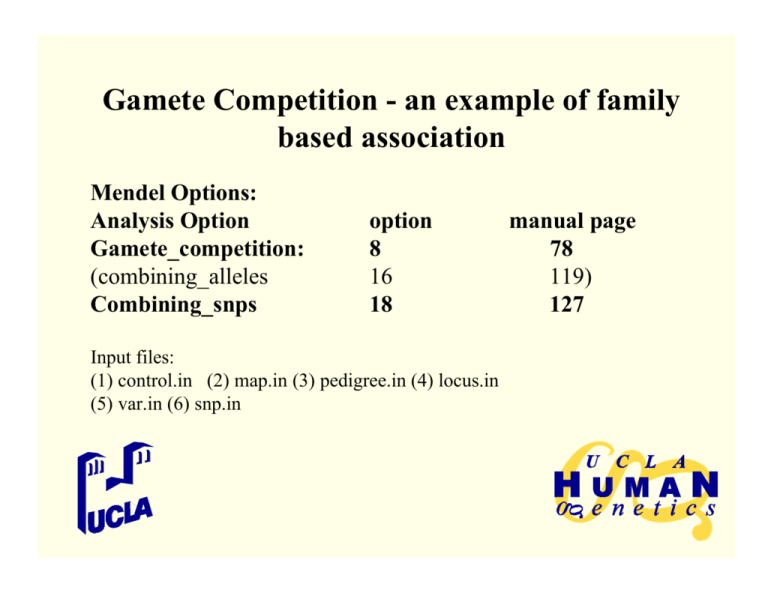
Gamete Competition - an example of family
based association
Mendel Options:
Analysis Option
Gamete_competition:
(combining_alleles
Combining_snps
option
8
16
18
Input files:
(1) control.in (2) map.in (3) pedigree.in (4) locus.in
(5) var.in (6) snp.in
manual page
78
119)
127
The gamete competition is an extension of
the TDT
What are the Limitations of the original TDT?
(1) Nuclear Families
(2) Qualitative traits
(3) Codominant markers
Lange (1988), Jin et al. (1994), and Sham and Curtis (1995)
considered a model (Bradley Terry, 1952) that was originally used
to predict the outcome of team sports.
Gamete Competition -Summary
(1) Gamete Competition works on extended pedigrees. No need to break up large
families into nuclear families.
(2) If the data are trios, the gamete competition and the TDT are equivalent.
Their null hypothesis is no linkage or no association. The alternative hypothesis is
linkage and association.
(3) When considering more than one affected per family, the TDT and gamete
competition confound association with linkage. When using only a small number
of very large families, the gamete competition will provide little new information
over a traditional linkage analysis.
(4) Exact p-values can be determined with the TDT. Gamete competition
asymptotic p-values are approximate.
(5) The gamete competition model can be used when there is missing marker
information. Allele frequencies can be fixed at population estimates or estimated
along with the transmission parameters.
(6) When there are missing data, the gamete competition is not immune to the
effects of population stratification or rare alleles.
Bradley - Terry Model of Competing
Sports Teams
In general for each team i, we assign a win parameter
τi so that the probability that i beats j is:
τi
P (i / j → i ) =
τi +τ j
Note that multiplying each τi by any a>0 does not
change its value, so one τi can be fixed at 1.
Note that if τi > τj for all j then i is the best team
How are sports competitions analogous to
the TDT?
(1) Each possible allele at locus = a team
(2) A heterozygous parent = a match up
(3) Allele received by child from a
heterozygous parent = the winner of the game
(4) The transmission parameters = the win parameters
(5) The win/lost record is determined by
the transmissions from heterozygous parents.
The gamete competition likelihood for a pedigree
The general form of the gamete competition likelihood for a
pedigree with n individuals is
L = ∑ ...∑∏ Pen( X i | Gi )∏ Prior (G j ) ∏ Tran (Gm | Gk , Gl )
G1
Gn i
j
{k ,l ,m}
Here person i has marker phenotype Xi and underlying marker
genotype Gi.
For founders genotypes probabilities = Prior(Gj)
For offspring, the transmission probability factors
Tran(Gm | Gk, Gl) = Tran(Gmk | Gk )*Tran(Gml | Gl )
Tran(Gml|Gl) are the Bradley-Terry probabilities if the child is affected.
They are the Mendelian probabilities otherwise.
The penetrance, Pen(Xi| Gi) is always 1 or 0, depending on
whether Xi and Gi are consistent or inconsistent
Assessing significance
We use a likelihood ratio test statistic
LRT = 2*( ln(LHa)-ln(LHo) )
Where LHa and LHo are the maximum likelihoods
under the alternative and null hypotheses.
Significance?
Approximate p-values can be calculated by assuming a
the distribution is chi-square or by gene dropping.
Toy Example: Complete Trios with One Affected
1
Not transmitted
1
--2
6
3
8
4
8
5
7
2
6
--5
7
8
transmitted
3
4
4
7
--7
6
4
5
5
--7
5
5
4
6
5
---
When we ignore disease status, the Bradley- Terry
model provides a form of segregation analysis.
When we consider the transmission to affected
members only (like this example) we have a form of
TDT analysis.
LRT = 3.63, the p-value of 0.46 supports acceptance
of the null hypothesis
Can this model be extended to quantitative
traits?
Yes by recognizing that the Bradley – Terry Model is equivalent to a matched
case control design. The transmitted allele is the case, the untransmitted allele
ωi x p
is the control.
i
τ =e
where xp denotes child p’s standardized trait value, i denotes allele i and
the probability of an i/j heterozygous parent transmitting i is
P(i / j → i ) =
e
e
(ω i −ω j ) x p
(ω i −ω j ) x p
Note that one ω is set to zero.
This is equivalent to conditional logistic regression.
+1
Quantitative Trait Example: ACE
High ACE concentration is associated with a deletion
within an intron of the ace gene.
eωinsertion xk
P(insertion / deletion → insertion ) = ωinsertion xk
+1
e
1
P(insertion / deletion → deletion) = ωinsertion xk
+1
e
P(insertion / deletion → deletion)
+ P (insertion / deletion → insertion) ≡ 1.0
mle
s.e. of mle
Ho: ωinsertion = 0
ωinsertion
-1.309
0.17
ωdeletion
0.00
fixed
Ha: ωinsertion ≠ 0
LRT = 83.01 Asymptotic p-value < 1 x 10-9