Finding Confidence Intervals with R
Data
Suppose we’ve collected a random sample of 10 recently graduated students and asked them
what their annual salary is. Imagine that this is the data we see:
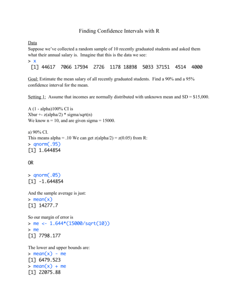
> x
[1] 44617 7066 17594 2726 1178 18898 5033 37151 4514 4000
Goal: Estimate the mean salary of all recently graduated students. Find a 90% and a 95%
confidence interval for the mean.
Setting 1: Assume that incomes are normally distributed with unknown mean and SD = $15,000.
A (1 - alpha)100% CI is
Xbar +- z(alpha/2) * sigma/sqrt(n)
We know n = 10, and are given sigma = 15000.
a) 90% CI.
This means alpha = .10 We can get z(alpha/2) = z(0.05) from R:
> qnorm(.95)
[1] 1.644854
OR
> qnorm(.05)
[1] -1.644854
And the sample average is just:
> mean(x)
[1] 14277.7
So our margin of error is
> me <- 1.644*(15000/sqrt(10))
> me
[1] 7798.177
The lower and upper bounds are:
> mean(x) - me
[1] 6479.523
> mean(x) + me
[1] 22075.88
So our 90% CI is ($6479, $22076.)
b. For a 95% CI, alpha = .05. All of the steps are the same, except we replace z(.05) with
z(.025)
> me <- qnorm(.975)*(15000/sqrt(10))
> me
[1] 9296.925
> mean(x) - me
[1] 4980.775
> mean(x) + me
[1] 23574.63
The new interval, (9296, 23574) is wider, but we are more confident that it contains the true
mean.
Setting II: Same problem, only now we do not know the value for the SD. Therefore, we must
estimate it from the data:
> sd(x)
[1] 15345.95
Now a (1-alpha)100% CI looks like
Xbar +- t(alpha/2, df) * s/sqrt(n)
We just calculated s = 15345 and n = 10 still. Xbar is still 14277.
1. 90% CI
Alpha = .10.
All we need is the t-value:
Because the degrees of freedom are n-1 = 10-1 = 9:
> qt(.95,9)
[1] 1.833113
> me <- qt(.95,9)*sd(x)/sqrt(10)
> me
[1] 8895.76
> mean(x) - me
[1] 5381.94
> mean(x) + me
[1] 23173.46
So the 90% CI is: (8896,23173). Note that this is wider than the last 90% CI.
2. 95% CI. Now alpha = .05.
> me <- qt(.975,9)*sd(x)/sqrt(10)
> me
[1] 10977.83
> mean(x) - me
[1] 3299.868
> mean(x) + me
[1] 25255.53
(3300,25255)
Note that the lower end is getting dangerously close to 0! Note that this is the widest interval
yet.
Setting III:
Now we no longer assume the data are normal. Note that a look at the histogram and the qqnorm
plot show that this wasn’t such a great assumption to begin with:
So at best, the confidence intervals from above are approximate. The approximation, however,
might not be very good.
A bootstrap interval might be helpful. Here are the steps involved.
1. From our sample of size 10, draw a new sample, WITH replacement, of size 10.
2. Calculate the sample average, called the bootstrap estimate.
3. Store it.
4. Repeat steps 1-3 many times. (We’ll do 1000).
5. For a 90% CI, we will use the 5% sample quantile as the lower bound, and the 95% sample
quantile as the upper bound. (Because alpha = 10%, so alpha/2 = 5%. So chop off that top and
bottom 5% of the observations.)
Here’s the R-code:
> bstrap <- c()
> for (i in 1:1000){
+ # First take the sample
+ bsample <- sample(x,10,replace=T)
+ #now calculate the bootstrap estimate
+ bestimate <- mean(bsample)
+ bstrap <- c(bstrap,bestimate)}
> #lower bound
> quantile(bstrap,.05)
5%
7413.795
> #upper bound
> quantile(bstrap,.95)
95%
21906.49
>
We use the same output to get the 95% confidence interval:
> #lower bound for 95% CI is the 2.5th quantile:
> quantile(bstrap,.025)
2.5%
6357.615
> quantile(bstrap,.975)
97.5%
23736.75
So the 90% CI is (7414,21906)
and the 95% is (6358,23737).
Note: this method of using the sample quantiles to find the
bootstrap confidence interval is called the Percentile Method.
There are other methods that might be more suitable for some
situations.
This code could be made much more streamlined:
> bstrap <- c()
> for (i in 1:1000){
+ bstrap <- c(bstrap, mean(sample(x,10,replace=T)))}
and then you find the quantiles as before.
You can also write a function that takes a data set (x), number of
bootstrap samples (B) as input:
bsci <- function(x,B){
bstrap <- c()
for (i in 1:B){
bstrap <- c(bstrap,mean(sample(x,length(x),replace=T)))}}
Now to find, say, a 95% CI we need only do:
> output <- bsci(x,1000)
> quantile(output,.025)
2.5%
6486.743
> quantile(output,.975)
97.5%
23768.4