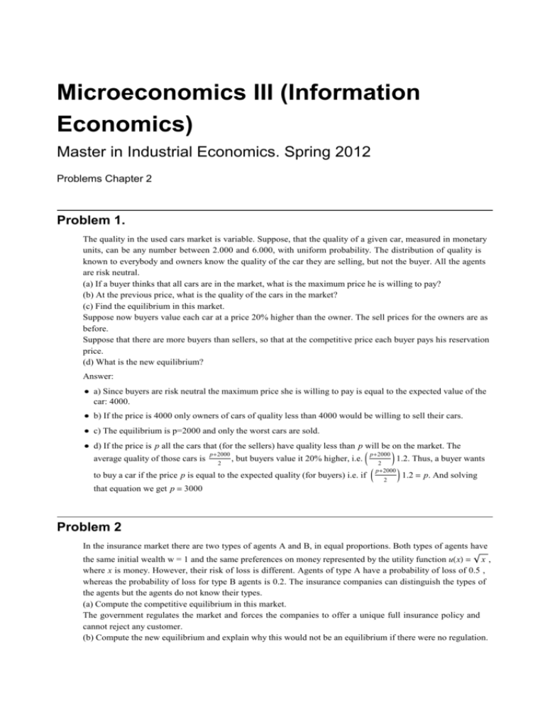
Microeconomics III (Information
Economics)
Master in Industrial Economics. Spring 2012
Problems Chapter 2
Problem 1.
The quality in the used cars market is variable. Suppose, that the quality of a given car, measured in monetary
units, can be any number between 2.000 and 6.000, with uniform probability. The distribution of quality is
known to everybody and owners know the quality of the car they are selling, but not the buyer. All the agents
are risk neutral.
(a) If a buyer thinks that all cars are in the market, what is the maximum price he is willing to pay?
(b) At the previous price, what is the quality of the cars in the market?
(c) Find the equilibrium in this market.
Suppose now buyers value each car at a price 20% higher than the owner. The sell prices for the owners are as
before.
Suppose that there are more buyers than sellers, so that at the competitive price each buyer pays his reservation
price.
(d) What is the new equilibrium?
Answer:
è a) Since buyers are risk neutral the maximum price she is willing to pay is equal to the expected value of the
car: 4000.
è b) If the price is 4000 only owners of cars of quality less than 4000 would be willing to sell their cars.
è c) The equilibrium is p=2000 and only the worst cars are sold.
è d) If the price is p all the cars that (for the sellers) have quality less than p will be on the market. The
average quality of those cars is
p+2000
2
, but buyers value it 20% higher, i.e. J
p+2000
to buy a car if the price p is equal to the expected quality (for buyers) i.e. if J
that equation we get p = 3000
N 1.2. Thus, a buyer wants
2
p+2000
2
N 1.2 = p. And solving
Problem 2
In the insurance market there are two types of agents A and B, in equal proportions. Both types of agents have
the same initial wealth w = 1 and the same preferences on money represented by the utility function uHxL = x ,
where x is money. However, their risk of loss is different. Agents of type A have a probability of loss of 0.5 ,
whereas the probability of loss for type B agents is 0.2. The insurance companies can distinguish the types of
the agents but the agents do not know their types.
(a) Compute the competitive equilibrium in this market.
The government regulates the market and forces the companies to offer a unique full insurance policy and
cannot reject any customer.
(b) Compute the new equilibrium and explain why this would not be an equilibrium if there were no regulation.
(c) Discuss the efficiency in each situation and, if possible, compare them.
2
whereas the probability of loss for type B agents is 0.2. The insurance companies can distinguish the types of
the agents but the agents do not know their types.
(a) Compute the competitive equilibrium in this market.
answersProblemCh2AdveSel2.nb
The government regulates the market and forces the companies to offer a unique full insurance policy and
cannot reject any customer.
(b) Compute the new equilibrium and explain why this would not be an equilibrium if there were no regulation.
(c) Discuss the efficiency in each situation and, if possible, compare them.
Answers:
è a) In this case firms will “reveal” the types of agents. They will offer different contracts to different types.
Say that the loss is equal to 1 (the precise number is not important). Type A agents will get full inusrance
with the contract (1,0.5) (the amount of insurance is 1 and the premium is 0.5). Type B agents will get full
insurance with the contract (1, 0.2). Notice that firms can’t cheat, i.e. if a firms offers to a type B person the
contract corresponding to the type A person, so that the firm makes a positive profit, other firms will offer
the type B contract and “steal” that consumer (perfect competition)
è b) In this case firms will use the average probability, 0.35, in their contracts. They will offer the contract (1,
0.35). Agents will accept it.
è c) we will discuss it in class
Problem 3
(Separating equilibrium in the model where “The principals compete for the agents”. Based on Exercise 22b in
Microeconomics by Thomas Nechyba ). Suppose a perfect competitve insurance market. Agents face the
possibility of a bad outcome in which their consumption is x1 and the possibility of a good outcome in which
their consumption is x2 . Suppose further that there are two consumer types, consumers of type ∆ facing outcome
x1 with probability ∆ and consumers of type Φ facing outcome x1 with probability Φ. We assume that ∆<Φ. Each
type knows the risk he or she faces but the insurance companies do not which type any given individuals
represents. Insurance companies know the fraction Γ of the population of type ∆ (and the remaining fraction
(1-Γ) is of type Φ). INsurance companies offer insurance contracts that are defined by an insurance premium p
and and insurance benefit b (if a consumer purchases an insurance contract Hp, bL, his or her consumption in the
good state is Hx2 - pL while his or her consumption in the bad state is Hx1 + b - pL. Suppose that the utility
function of the agents is uHxL = Α lnHxL. Suppose that x1 = 10, x2 = 250, ∆ = 0.25 and Φ = 0.5.
è Find the contracts Hp∆ , b∆ L, IpΦ , bΦ M that can be a separating equilibrium in this market.
è Can you say something about how the equilibrium insurance contract for the low risk type ∆ changes as the
high type becomes riskier. i.e. as Φ increases?
Answer :
We know that the type Φ agent will get (actuarily fair) full insurance. This implies a consumption level of
HH1 - ΦL x2 + Φx1 L with certainty. The full insurance utility for type Φ is U Φ = ΑlnHH1 - ΦL x2 + Φx1 L. The indifference curve that gives all combinations of b and p such that Φ type is indifferent to the full insurance outcome is
then given by
ΦΑlnHx1 + b - pL + H1 - ΦL ΑlnHx2 -p)=ΑlnHH1 - ΦL x2 + Φx1 L
we can solve for b to get
b=J
H1-ΦL x2 + Φ x1
Hx2 -pLH1-ΦL
N
1Φ
+ p - x1
Next we need to find the intersection of the above indifference curve with the line p = ∆b that represents the
menu of actuarily fair insurance contracts for type ∆ agent. Thus we need to solve
J
H1-ΦL x2 + Φ x1
Hx2 -pLH1-ΦL
N
1Φ
+ p - x1 =4p
which can be written as
1302
250-p
+ p - 10 = 4 p
and using the quadratic formula we get the equilibrium insurance contract for type ∆ (take the first root)
p = 21.30 and b = 4 p = 85.20
answersProblemCh2AdveSel2.nb
0.5 * 250 + 0.5 * 10
sol1 = SolveA
3
2
H250 - pL0.5
+ p - 10 - b Š 0, pE;
Plot@80.5 * b, 0.25 * b, p . sol1@@1, 1DD<, 8b, 10, 400<, AxesLabel ® 8b, p<D
p
200
150
100
50
100
200
300
400
b
You can check that as we increase Φ the equilibrium contract for type ∆ is such that the premium and the benefit
both go down. The next plot shows the equilibrium contracts for type ∆ when Φ goes from Φ=1 to Φ=0.25:
pes = TableAFindRootA
H1 - ΦL * 250 + Φ * 10
1Φ
H250 - pLH1-ΦL
+ p - 10 - 4 * p Š 0, 8p, 0<E,
8Φ, 0.25, 1, 0.05<E; fi = Table@i, 8i, 0.25, 1, 0.05<D; ListPlot@
Table@8Hp . pes@@iDDL 4, p . pes@@iDD<, 8i, 1, Length@pesD<D, AxesLabel ® 8b, p<D
p
60
50
40
30
20
10
50
100
150
200
b
4
answersProblemCh2AdveSel2.nb
TableForm@Table@8fi@@iDD, Hp . pes@@iDDL 4, p . pes@@iDD<, 8i, 1, Length@pesD<D,
TableHeadings ® 8None, 8"Φ", "b", "p"<<D
Φ
0.25
0.3
0.35
0.4
0.45
0.5
0.55
0.6
0.65
0.7
0.75
0.8
0.85
0.9
0.95
1.
b
240.
139.006
117.038
103.647
93.6108
85.1939
77.6058
70.4122
63.3362
56.174
48.7524
40.9008
32.4265
23.0809
12.4949
0.
p
60.
34.7515
29.2594
25.9117
23.4027
21.2985
19.4014
17.603
15.834
14.0435
12.1881
10.2252
8.10664
5.77022
3.12373
0.
More problems:
Problem 4. (exercise 1, page 160, of the book by Ines Macho Stadler and Perez Castrillo)
Problem 5. (exercise 2, page 160, of the book by Ines Macho Stadler and Perez Castrillo)
Problem 6. (exercise 3, page 161, of the book byInes Macho Stadler and Perez Castrillo)
Problem 7. (exercise 4, page 161, of the book by Ines Macho Stadler and Perez Castrillo)
Problem 8. (exercise 6, page 162, of the book by Ines Macho Stadler and Perez Castrillo)
Solutions: See the textbook