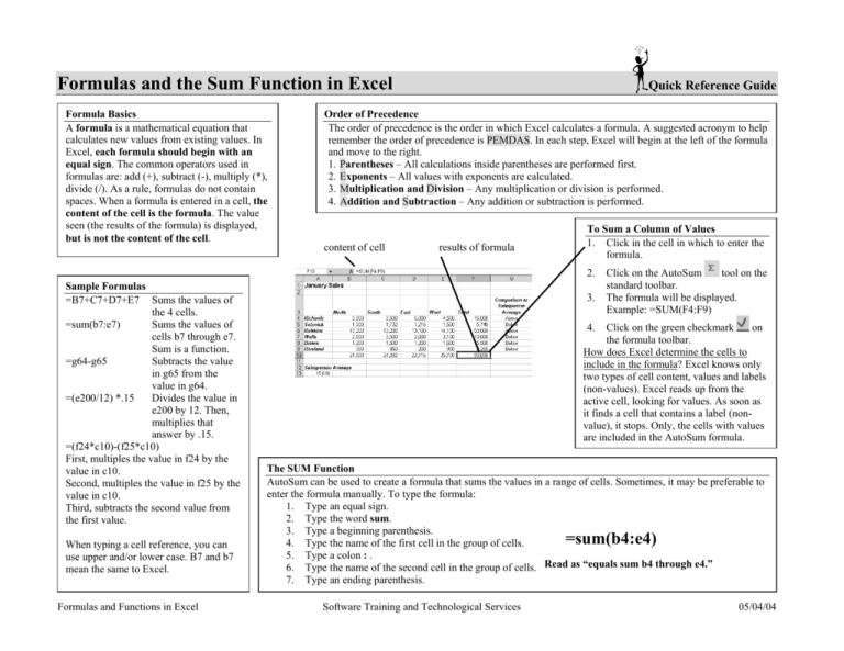
Formulas and the Sum Function in Excel
Formula Basics
A formula is a mathematical equation that
calculates new values from existing values. In
Excel, each formula should begin with an
equal sign. The common operators used in
formulas are: add (+), subtract (-), multiply (*),
divide (/). As a rule, formulas do not contain
spaces. When a formula is entered in a cell, the
content of the cell is the formula. The value
seen (the results of the formula) is displayed,
but is not the content of the cell.
Quick Reference Guide
Order of Precedence
The order of precedence is the order in which Excel calculates a formula. A suggested acronym to help
remember the order of precedence is PEMDAS. In each step, Excel will begin at the left of the formula
and move to the right.
1. Parentheses – All calculations inside parentheses are performed first.
2. Exponents – All values with exponents are calculated.
3. Multiplication and Division – Any multiplication or division is performed.
4. Addition and Subtraction – Any addition or subtraction is performed.
content of cell
results of formula
To Sum a Column of Values
1. Click in the cell in which to enter the
formula.
2.
Sample Formulas
=B7+C7+D7+E7 Sums the values of
the 4 cells.
=sum(b7:e7)
Sums the values of
cells b7 through e7.
Sum is a function.
=g64-g65
Subtracts the value
in g65 from the
value in g64.
=(e200/12) *.15
Divides the value in
e200 by 12. Then,
multiplies that
answer by .15.
=(f24*c10)-(f25*c10)
First, multiples the value in f24 by the
value in c10.
Second, multiples the value in f25 by the
value in c10.
Third, subtracts the second value from
the first value.
When typing a cell reference, you can
use upper and/or lower case. B7 and b7
mean the same to Excel.
Formulas and Functions in Excel
3.
tool on the
Click on the AutoSum
standard toolbar.
The formula will be displayed.
Example: =SUM(F4:F9)
4.
Click on the green checkmark
on
the formula toolbar.
How does Excel determine the cells to
include in the formula? Excel knows only
two types of cell content, values and labels
(non-values). Excel reads up from the
active cell, looking for values. As soon as
it finds a cell that contains a label (nonvalue), it stops. Only, the cells with values
are included in the AutoSum formula.
The SUM Function
AutoSum can be used to create a formula that sums the values in a range of cells. Sometimes, it may be preferable to
enter the formula manually. To type the formula:
1. Type an equal sign.
2. Type the word sum.
3. Type a beginning parenthesis.
=sum(b4:e4)
4. Type the name of the first cell in the group of cells.
5. Type a colon : .
6. Type the name of the second cell in the group of cells. Read as “equals sum b4 through e4.”
7. Type an ending parenthesis.
Software Training and Technological Services
05/04/04
Common Functions in Excel
Function Basics
A function has three parts:
a. Equal sign
b. Function name
c. Argument, enclosed in parentheses
Quick Reference Guide
=average(f4:f9)
There are no spaces in the
formula.
Examples of Functions to Count
COUNTA
Use this function to count the
number of cells that contain data (are not empty)
in the range specified within the parentheses.
Example: =COUNTA(A2:A653)
COUNT
This function counts the number
of cells that contain numbers (including values
that are the result of formulas), dates or numbers
stored as text in the range specified within the
parentheses. Example: =COUNT(C2:C653)
COUNTIF
Use this function to count the
number of cells in the range specified that meet
the criterion. The example formula would count
the number of cells in the range E2 through E 653
that have the contents M.
Example: =COUNTIF(E2:E653,“M”)
Additional examples of COUNTIF:
=COUNTIF(C2:C653,“>=3.25”) This formula
counts the number of cells within the range that
have a value greater than or equal to 3.25.
=COUNTIF(A2:C200,“”) This formula counts
the number of cells within the range that have
no data. There is no character, no space
between the quotation marks.
Ranges
Many formulas contain ranges, which are
groups of cells that have common boundaries
and form a rectangle in shape. Ranges may
contain cells in a single row, a single column or
may span several rows and columns. When
typing a range, the range name is from the top
left cell reference to the bottom right cell
reference. A colon is entered between the first
and the second cell reference. The colon is read
as “through.” Some examples of ranges are:
G4:G9 (G4 through G9)
B4:E9 (B4 through E9)
3-D Formulas
With multiple worksheets, some of the
formulas may include values that are stored on
different worksheets. A formula that references
cells on more than one worksheet is using 3D
references. The formula is called a 3D
formula. In a 3D formula, the cell reference
will include the sheet name. For example, this
formula sums the monthly totals for Richards,
which are on sheet1 in cell B4, on sheet 2 in
cell B4 and on sheet 3 in cell B4.
=sheet1!B4+sheet2!B4+sheet3!B4
In a 3-D formula, a cell is referenced by its
sheet and cell name. Sheet1!B4 is cell B4 on
sheet1. An exclamation point is used to
separate the sheet name from the cell name.
Help with Formulas
From the menu, click on Help, Microsoft Excel
Help. In the Search box, type examples of
formulas and click on the Search button.
Formulas and Functions in Excel
Help with Excel Functions
From the menu, click on Help, Microsoft
Excel Help. In the Search box, type functions
and click on the Search button.
Software Training and Technological Services
05/04/04