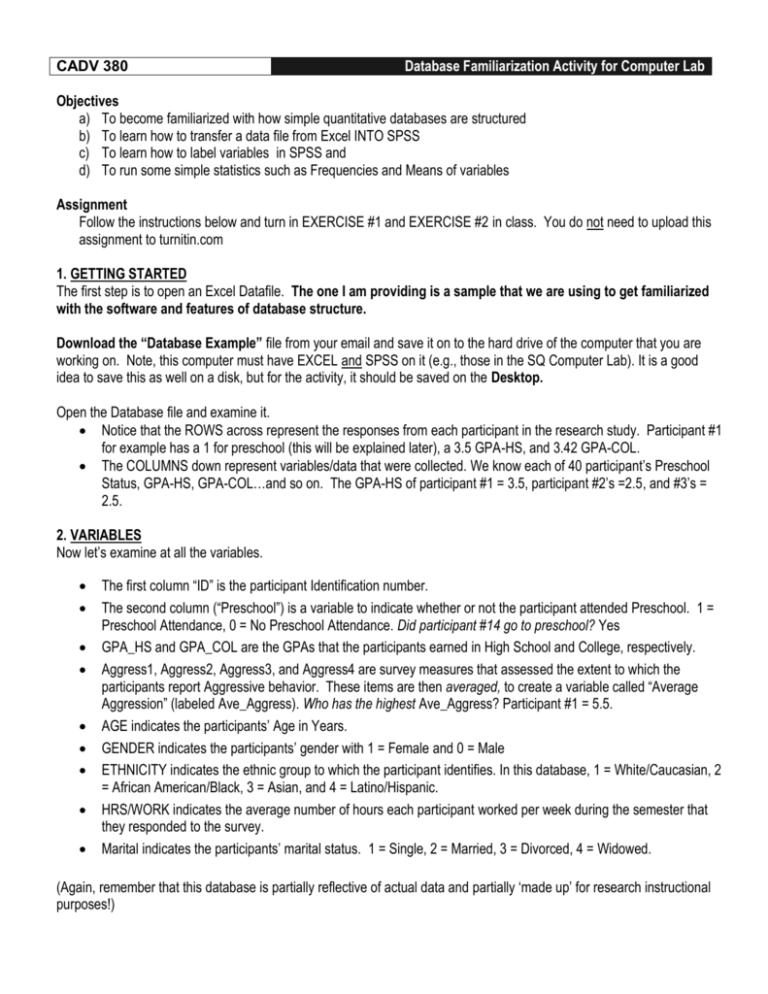
CADV 380
Database Familiarization Activity for Computer Lab
Objectives
a) To become familiarized with how simple quantitative databases are structured
b) To learn how to transfer a data file from Excel INTO SPSS
c) To learn how to label variables in SPSS and
d) To run some simple statistics such as Frequencies and Means of variables
Assignment
Follow the instructions below and turn in EXERCISE #1 and EXERCISE #2 in class. You do not need to upload this
assignment to turnitin.com
1. GETTING STARTED
The first step is to open an Excel Datafile. The one I am providing is a sample that we are using to get familiarized
with the software and features of database structure.
Download the “Database Example” file from your email and save it on to the hard drive of the computer that you are
working on. Note, this computer must have EXCEL and SPSS on it (e.g., those in the SQ Computer Lab). It is a good
idea to save this as well on a disk, but for the activity, it should be saved on the Desktop.
Open the Database file and examine it.
 Notice that the ROWS across represent the responses from each participant in the research study. Participant #1
for example has a 1 for preschool (this will be explained later), a 3.5 GPA-HS, and 3.42 GPA-COL.
 The COLUMNS down represent variables/data that were collected. We know each of 40 participant’s Preschool
Status, GPA-HS, GPA-COL…and so on. The GPA-HS of participant #1 = 3.5, participant #2’s =2.5, and #3’s =
2.5.
2. VARIABLES
Now let’s examine at all the variables.









The first column “ID” is the participant Identification number.
The second column (“Preschool”) is a variable to indicate whether or not the participant attended Preschool. 1 =
Preschool Attendance, 0 = No Preschool Attendance. Did participant #14 go to preschool? Yes
GPA_HS and GPA_COL are the GPAs that the participants earned in High School and College, respectively.
Aggress1, Aggress2, Aggress3, and Aggress4 are survey measures that assessed the extent to which the
participants report Aggressive behavior. These items are then averaged, to create a variable called “Average
Aggression” (labeled Ave_Aggress). Who has the highest Ave_Aggress? Participant #1 = 5.5.
AGE indicates the participants’ Age in Years.
GENDER indicates the participants’ gender with 1 = Female and 0 = Male
ETHNICITY indicates the ethnic group to which the participant identifies. In this database, 1 = White/Caucasian, 2
= African American/Black, 3 = Asian, and 4 = Latino/Hispanic.
HRS/WORK indicates the average number of hours each participant worked per week during the semester that
they responded to the survey.
Marital indicates the participants’ marital status. 1 = Single, 2 = Married, 3 = Divorced, 4 = Widowed.
(Again, remember that this database is partially reflective of actual data and partially ‘made up’ for research instructional
purposes!)
** HOLD ON -- LET’S REVIEW TYPES OF VARIABLES **
There are two general types of variables that we will consider -- Continuous and Categorical variables.

Continuous variables -- A continuous variable has numeric values such as 1, 2, 3.14, -5, etc. The relative
magnitude of the values is significant (e.g., a value of 2 indicates twice the magnitude of 1, 4 is twice as big as 2).
Examples of continuous variables are blood pressure, height, weight, income, age, and probability of illness.
o What variables in this database are continuous? GPAs, Aggression, Age, Hours worked.

Categorical variables -- A categorical variable has values that function as labels rather than as numbers. Some
programs call categorical variables “nominal” variables. For example, a categorical variable for gender might use
the value 1 for male and 2 for female (or any other two numbers). The actual magnitude of the value is not
significant; coding male as 7 and female as 3 would work just as well. As another example, marital status might
be coded as 1 for single, 2 for married, 3 for divorced and 4 for widowed.
o What variables in this database are categorical? Preschool, Gender, Ethnicity, Marital status.
3. TRANSFERRING FILES ONTO SPSS
Now that you are familiarized with the layout of the database in Excel, you will need to TRANSFER the database over to
an SPSS format in order to be able to run analyses. In order to do this, you need to first CLOSE THE EXCEL
DATABASE FILE you have been looking at. Save and close the file.
Now you need to OPEN SPSS:
a.
To open SPSS, go to START ALL PROGRAMS SPSSSPSS14 FOR WINDOWS)
b. Now, SPSS is open and you should be looking at a blank spreadsheet (If a dialog box opens up click “CANCEL”).
You want to import your Excel data. Click on “FILE” then “OPEN” then “DATA”. A dialog box should open up.
On the top option box, Look in: DESKTOP. On the bottom option box for “Files of type” (if using Windows) or
“enable” if using Mac, select the Excel (*.xls) file type. Then select the folder on the (Desktop) that your file is
saved in and find the file name. Click “OPEN”. The SPSS program will ask you if the first row of data indicates
the variable names - Click “OK” to continue on and it should open up a new window with SPSS and your data
imported into it.
4. LABELING OUR VARIABLES
Now we get to play 
Double click on “ID” and the screen will turn into the “Variable View”. (You can also do this by clicking on the tab at the
lower left of the screen that says “VARIABLE VIEW”. This will allow you to re-name or label the variables.
If you click in any of the cells under the column called “Values”, there should be a little grey box that shows up on the right
edge. Click on this box and you can specify the value of the given variable. If you click on “Value” box in the 2nd row
(Preschool row) then you can label, “0” (for Value) and “No Preschool” for the corresponding “Label” then click “ADD” to
enter it. Now, type in “1” for the next value and “Preschool” for the label. Click “ADD” and “Continue” to close the box
(TRY THIS)
(By labeling the value options, then if/when you run analyses or graph the results, the variables will be labeled
appropriately to the conditions you specified.)
Click on the Value column for the row called “Gender” and label the values as 0 for Male and 1 for Female.
(You can label the Ethnicity and Marital variables as well according the group descriptions on the previous page.)
Click on DATA VIEW at the bottom left of the screen to get back to the dataset view.
** HOLD ON -- LET’S REVIEW FREQUENCIES **
A frequency table is used to summarize categorical, nominal, and ordinal data. It is a record of how often each value (or
set of values) of the variable in question occurs. It may also report the percentages that fall into each category. Say we
wanted to know how many Males and Females we had in our dataset – this is asking for the frequency of each gender.
We could go through and count each one by hand to get this frequency information or we could run a frequency analysis.
5. RUNNING SIMPLE FREQUENCIES (FOR CATEGORICAL VARIABLES)
1) On the top toolbar, Click on ANALYZE  DESCRIPTIVE STATISTICS  FREQUENCIES
2) Double click over the variable name (i.e., preschool) to move it into the dialog box on the right (you can also
single click and use the arrow) and then click “OK”.
3) A new window will open (called “output”). Here you can see how many participants are in each of your groups.
You can do this to determine the frequency of any of your variables (This is usually done for categorical variables
– think about what would happen if you did this for a continuous variable. Try it if you’d like).
** HOLD ON -- LET’S REVIEW MEANS **
The central tendency of a distribution is an estimate of the "center" of a distribution of values. There are three major types
of estimates of central tendency: Mean, Median and Mode. The mean or average is probably the most commonly used
method of describing central tendency. To compute the mean all you do is add up all the values and divide by the number
of values. For example, the mean or average quiz score is determined by summing all the scores and dividing by the
number of students taking the exam. You can then look at one individual quiz score and see if it is above or below the
class average or mean.
6. FINDING MEANS FOR VARIABLES (FOR CONTINUOUS VARIABLES)
If you want to know what the mean is of a continuous variable (on a ratio or interval scale), you would follow the same
procedure, except you would click, ANALYZE  DESCRIPTIVE STATISTICS  DESCRIPTIVES and click over the
variable. What is the mean high school GPA for our sample? 3.237 (Why wouldn’t we run means for categorical
variables?)
** HOLD ON -- LET’S REVIEW P-VALUES **
Remember the null hypotheses – the hypothesis that there is no difference. Each statistical test has an associated null
hypothesis – there is no difference between your groups (or whatever you are comparing). The p-value is the probability
that the null hypothesis is TRUE (there is no difference) and any difference that you do see is by sheer chance. How
much of a chance? That depends on the magnitude of the p-value. A p-value of .05, for example, indicates that you
would have only a 5% chance of drawing the sample being tested if the null hypothesis was actually true – there is only a
5% chance that any differences you see are by chance alone, no relationship or true differences.
A p-value close to zero signals that your null hypothesis is false, and typically that a difference is very likely to exist. Large
p-values closer to 1 imply that there is no detectable difference for the sample size used (1 = 100% probability of any
differences being due to chance alone).
A p-value of 0.05 is a typical threshold used to evaluate the null hypothesis most fields. Say you wanted to know the
likelihood of an immunization being the cause of death in children. Would p < .05 be an adequate level of certainty for
you?
7. RUNNING A T-TEST
SCENARIO A - If you have an independent variable where you have two groups, and a dependent variable that is
continuous, then you will want to use a T-test (don’t worry about what this stands for). (In our database, an example of
this would be if you want to examine whether there are differences in GPA-COL, based on whether a person attended
Preschool or not. IV would be Preschool, DV would be GPA-COL).
Select ANALYZECOMPARE MEANSINDEPENDENT SAMPLES T-TEST->
Under The “TEST” variable, click over your dependent variable. Under the “GROUPING” variable, click over your
independent variable.
Click “Define Groups” and specify the values that you assigned for the groups (1 and 0) Then click ‘ok’ for it to run the ttest. Now view your output and check it with the DATABASE ACTIVITY ANSWER SHEET.
Now might be a good time to do EXERCISE #1
8. RUNNING AN ANOVA
SCENARIO B - If you have an independent variable where you have three or more groups, and a dependent variable
that you measure on an interval or ratio scale, then you will want to use an ANALYSIS OF VARIANCE (also known as
the ANOVA F-test). (In the database example, this would be if you wanted to examine if there are differences in the
amount of hours worked based on different ethnic groups. IV would be Ethnicity, DV would be hours worked, and you
would run an ANOVA.
Select ANALYZECOMPARE MEANSONEWAY ANOVA > Under the DEPENDENT list, click over your dependent
variable. Under the “factor”, click over your independent variable. Click on OPTIONS and make sure the box marked
“Descriptives” is checked and Click “Continue”. Click “OK” to run the Analysis. Now view your output and check it with the
DATABASE ACTIVITY ANSWER SHEET.
Now might be a good time to do EXERCISE #2
ANALYSIS CHART
Below is a summary of different types of analyses required depending on the type of data that you would like to analyze.
You many find this useful as you plan the analyses for your research proposal.
Dependent Variable
Independent
Variable
Categorical
Continuous
Categorical (2 levels)
Chi-square
T-test
Categorical (> 2 levels)
Chi-square
ANOVA
Continuous
Logistic regression
Correlation or
Regression
EXERCISE #1
1. Perform a T-test that examines the high school GPA of participants that went to preschool compared to those that did
not go to preschool. (Hint: IV = Preschool, DV = GPA-HS)
2. Print your output and label the means, t-statistic, and p-value (indicate whether or not it is significant).
EXERCISE #2
1. Perform an ANOVA that examines whether or not hours worked differs with marital status. (Hint: IV = Marital DV =
hrswork)
2. Print your output and label the means and p-value (indicate whether or not it is significant).