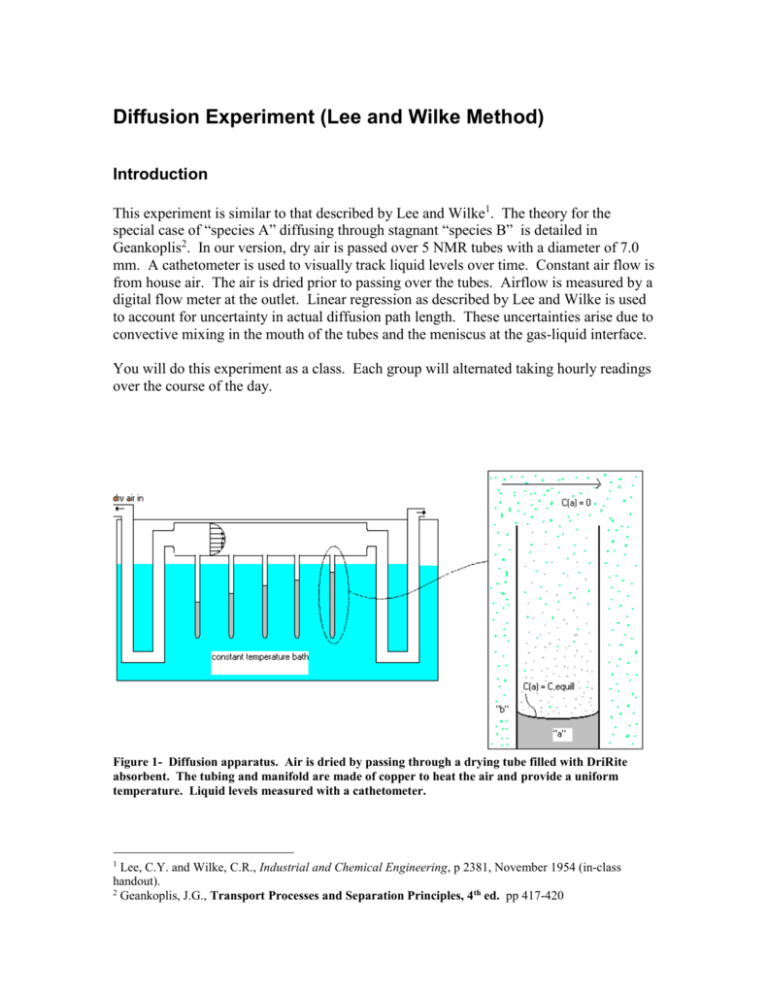
Diffusion Experiment (Lee and Wilke Method)
Introduction
This experiment is similar to that described by Lee and Wilke1. The theory for the
special case of “species A” diffusing through stagnant “species B” is detailed in
Geankoplis2. In our version, dry air is passed over 5 NMR tubes with a diameter of 7.0
mm. A cathetometer is used to visually track liquid levels over time. Constant air flow is
from house air. The air is dried prior to passing over the tubes. Airflow is measured by a
digital flow meter at the outlet. Linear regression as described by Lee and Wilke is used
to account for uncertainty in actual diffusion path length. These uncertainties arise due to
convective mixing in the mouth of the tubes and the meniscus at the gas-liquid interface.
You will do this experiment as a class. Each group will alternated taking hourly readings
over the course of the day.
Figure 1- Diffusion apparatus. Air is dried by passing through a drying tube filled with DriRite
absorbent. The tubing and manifold are made of copper to heat the air and provide a uniform
temperature. Liquid levels measured with a cathetometer.
1
Lee, C.Y. and Wilke, C.R., Industrial and Chemical Engineering, p 2381, November 1954 (in-class
handout).
2
Geankoplis, J.G., Transport Processes and Separation Principles, 4th ed. pp 417-420
Standard Operating Procedure
1. You will be given a bottle of either acetone or cyclohexane to use for this
experiment. Check the MSDR for hazards of these substances. Use appropriate
PPE (safety glasses and nitrile rubber gloves).
2. Use the syringe and fill tube provided to fill the NMR tubes to five different
levels of your choosing. Fill from the bottom so as to keep surfaces above the
liquid level from being wetted.
3. Insert tubes in the manifold such that they are all aligned perpendicular to the air
flow and protrude into the manifold the same distance.
4. Place the manifold into the constant temperature bath (aquarium) and fill the bath
to within one centimeter of the manifold (after the bath is heated you may top off
the fluid so that it is within a few millimeters if the manifold).
5. Set the bath to the desired temperature and set the airflow to the desired rate and
allow tocome to equilibrium.
6. Level the cathetometer using the thumbscrews on the feet of the device. Use duct
tape to secure the cathetometer to the floor so that it is less likely to move if
accidentally bumped.
7. Level the telescope using the thumbscrew on the scope.
8. Carefully take initial level measurements of all tubes by adjusting the height of
the scope using the thumbscrew that controls the height (note that the readings are
Repeat once per hour for 6 hours. Use extreme caution when adjusting the height
during the day- if the apparatus is handled roughly or bumped, your
measurements will not be accurate. Note that the final significant figure of your
height is read from the Vernier scale. See http://en.wikipedia.org/wiki/Vernier for
instructions on reading Vernier scales.
9. Repeat this experiment at a new temperature on day 2.
Analysis
1. Calculate the apparent diffusivity for each tube using eqn. 6.2-262. Plot your data
by modifying equation 6.26-26 in such a way that all of the time data is used and
the diffusion coefficient may be obtained from the inverse slope. Is the data
linear- are there any patterns? Why or why not? How long would you expect it to
take for the system to come to steady state? What does scatter in the data
represent? Use linear regression and statistical output (Excel or Polymath) to
estimate the uncertainty in the value of diffusivity based solely on the the
assumption of random scatter in the data.
2. Plot the apparent diffusivity values of each tube as in eqn 11 in Lee and Wilke in
order to determine actual values of diffusivity. Use linear regression and statistical
output (Excel or Polymath) to estimate the uncertainty in the value of diffusivity
based solely on the the assumption of random scatter in the data.
3. Calculate the expected value of diffusivity using both the Chapman-Enskog
equation (6.2-44) and the Fuller, Schettler and Giddings method (eqn 6.2-45, table
6.2-2 in Geankoplis).
4. Compare your experimental value of the diffusivity coefficient with the estimated
values from number 2 above, as well as with the literature value for aircyclohexane or air-acetone. Are the results consistent? Is the temperature
dependence between T1.5 and T1.75?
5. What systematic uncertainties are present as a result of the methods and materials
you used to measure the diffusion coefficient?
6. What assumptions were made in the derivation of equation 6.2-26? How does the
method outlined in the Lee and Wilke paper correct for some of the “nonidealities” of the system? (explain fully)
7. Show plots in items 1 and 2 in your “Results” section and discuss all items fully
in the “Discussion”.