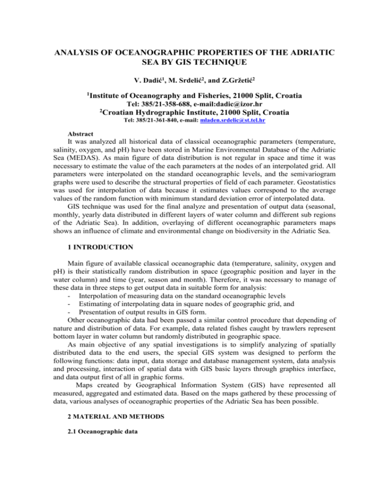
ANALYSIS OF OCEANOGRAPHIC PROPERTIES OF THE ADRIATIC
SEA BY GIS TECHNIQUE
V. Dadić1, M. Srdelić2, and Z.Gržetić2
1
Institute of Oceanography and Fisheries, 21000 Split, Croatia
Tel: 385/21-358-688, e-mail:dadic@izor.hr
2
Croatian Hydrographic Institute, 21000 Split, Croatia
Tel: 385/21-361-840, e-mail: mladen.srdelic@st.tel.hr
Abstract
It was analyzed all historical data of classical oceanographic parameters (temperature,
salinity, oxygen, and pH) have been stored in Marine Environmental Database of the Adriatic
Sea (MEDAS). As main figure of data distribution is not regular in space and time it was
necessary to estimate the value of the each parameters at the nodes of an interpolated grid. All
parameters were interpolated on the standard oceanographic levels, and the semivariogram
graphs were used to describe the structural properties of field of each parameter. Geostatistics
was used for interpolation of data because it estimates values correspond to the average
values of the random function with minimum standard deviation error of interpolated data.
GIS technique was used for the final analyze and presentation of output data (seasonal,
monthly, yearly data distributed in different layers of water column and different sub regions
of the Adriatic Sea). In addition, overlaying of different oceanographic parameters maps
shows an influence of climate and environmental change on biodiversity in the Adriatic Sea.
1 INTRODUCTION
Main figure of available classical oceanographic data (temperature, salinity, oxygen and
pH) is their statistically random distribution in space (geographic position and layer in the
water column) and time (year, season and month). Therefore, it was necessary to manage of
these data in three steps to get output data in suitable form for analysis:
- Interpolation of measuring data on the standard oceanographic levels
- Estimating of interpolating data in square nodes of geographic grid, and
- Presentation of output results in GIS form.
Other oceanographic data had been passed a similar control procedure that depending of
nature and distribution of data. For example, data related fishes caught by trawlers represent
bottom layer in water column but randomly distributed in geographic space.
As main objective of any spatial investigations is to simplify analyzing of spatially
distributed data to the end users, the special GIS system was designed to perform the
following functions: data input, data storage and database management system, data analysis
and processing, interaction of spatial data with GIS basic layers through graphics interface,
and data output first of all in graphic forms.
Maps created by Geographical Information System (GIS) have represented all
measured, aggregated and estimated data. Based on the maps gathered by these processing of
data, various analyses of oceanographic properties of the Adriatic Sea has been possible.
2 MATERIAL AND METHODS
2.1 Oceanographic data
Oceanographic investigation in the Adriatic Sea has been done for more than a century
by many institutions from Croatia, as well as many international oceanographic organizations.
It includes physical oceanography, chemistry, biology and fisheries. Classical oceanographic
parameters represent the most often measured oceanographic parameters. As data had been
collected by many institutions and measured at various sea levels using different methods and
instruments (BOT - bottle data, MBT - mechanical bathythermograph, XBT – expanded
bathythermograph, CTD - multiparametar probe), data quality control (QC) has been one of
major task. After QC procedure that included duplicate elimination, range checking,
statistical checks and static stability check of data more data were excluded from processing,
e.g. 49% of BOT data and 8% of MBT data (Table 1).
Main figure of data distribution is not regular in space and time (Fig. 1). They had been
collected at various (statistically random) sea levels, geographic positions (oceanographic
stations) and seasons during year depending of used methods and purpose of measurements.
Table 1 Number of classical oceanographic data received from different countries
/projects and number of unique and correct data
Temperature (oC)
Salinity (psu)
BOT
MBT
XBT
CTD
BOT
CTD
Oxygen
(ml/l)
pH
Croatia
27934
25693
0
834
22524
834
5394
2138
Italy
8372
0
0
275
5612
275
974
293
Data source
USA
6618
2137
2436
162
4517
162
1094
895
Greece
0
0
0
1356
0
1356
0
0
MEDAR
9488
1142
553
2241
8488
2241
0
0
MODAB
4036
638
0
174
2504
2174
0
0
Russia
3840
375
0
0
1314
0
0
0
France
1398
0
0
0
1225
0
185
63
Total
61686
29985
2989
5042
46184
7042
7647
3389
Unique and
correct data
31279
27496
2737
1352
28722
3841
5840
2925
50.7
91.7
91.5
26.8
62.2
54.5
76.3
86.0
(%)
A)
B)
Fig. 1 Number of measured data by year (A) and spatial distribution of station in the Adriatic Sea
(B)
2.1 Method of interpolation data on standard levels
There are more so call general and local methods of interpolation. Local interpolation
methods take into account only neighborhood data and it is more suitable for applications
data on the standard levels because water has completely different properties in specific parts
of water column. There are more local methods of interpolations (Ratrray, 1958; Reigein and
Ross, 1964, Dadic, 1996). In this paper second order Newton’s method of finite differences
from three unequally spaced positions instead Langange’s method. This method determines
the interpolated value pijk (x0) and its errors Rijk(x0).
Let us take values of the dependent variable y1, y2, y3, y4 to be known at successive
positions x1, x2, x3, x4 where x4>x3>x0>x2>x1. Then the value of y0 at position x0 lying
between x2 and x3 is
y0= pijk (x0) +Rijk(x0), where pijk(x)=yi + k1(x-xi)+ k2 (x-xi)(x-xj), and
k1= xj-xi =(yj-yi)/( xj-xi, k2= xj,xi,xk = xj-kk - xj-kk / xj-kk,
with i, j, k equal to either 1,2,3 or 2,3,4, respectively.
This formula was improved according Reiniger and Ros introducing a reference curve to
minimize the effect of unacceptable parabola on the final interpolated values. It is created by
adjusting the linearly interpolated value by an amount related to the difference between the
interpolated value (two inner points) and extrapolated value (two outer points). It is used a
weighting which is inversely proportional to some power of the separations between the
interpolated and extrapolated points. According Dadic, 2001 the best-fitted reference curve
for classical oceanographic parameters has the form:
1
yR.(x) = y23+(y12-y23)1.5y34+(y23-y34)1.5 y12 / (y12-y23)1.5 +(y23-y34)1.5
2
Interpolation y(x) includes linear interpolation between the values obtained from two
parabola (Fig. 2.A) and the reference curve yR.(x) (Fig. 2.B) as in formula:
y(x) = (yR-yp1)0.6yp2 + (yR-yp2)0.6 yp1 / (yR-yp1)0.6 +(yR-yp2) 0.6,
0
0
1
A)
1
1
0
2
2
0
Dubina(m)
Dubina(m)
Measuring levels:
1, 2, 3 4
2
D -2
0
e
pt
h
3
0
 
3
0
3
4
0
3
7
.
7
3
7
.
8
Interpolation point 
Extrapolation point 
Measuring level

3
4
0
Standard level
5
0
3
7
.
6
B)
1
0
4
4
3
7
.
9
3
8
.
0
S
la
n
o
s
t(
p
p
t
)
Salinity
(ppt)
3
8
.
1
3
8
.
2
5
0
8
.
3
3
7
.3
6
3
7
.7
3
7
.8
3
7
.9
3
8
.0
Salinity (ppt)
S
la
n
o
s
t(
p
p
t)
3
8
.1
3
8
.2
Fig. 2 Procedure of local interpolation on the standard oceanographic levels using
second order of Newton’s method (A) corrected by linear reference curve (B).
For the top and bottom of water column where there is only one point above or below
standard level it is necessary to adopt this formula for linear interpolation. This formula gives
less reliable results than in the interior of water column because the curve is almost
completely dominated by information below or above the region of interpolation.
An automatic software tools was developed for interpolation data from observed to
standard oceanographic levels with graphic visualization of output results (interpolated value
and expected error). All data profiles were passed through quality control before and after
3
8
.3
their interpolation on standard levels. Values of all parameters have to be inside of minimum
and maximum, as well as climatological range.
2.2 Method of geostatistical analysis and presentation of spatially distributed data
Geostatistical analysis represents an application of probability theory to estimate statistics
relating to spatial variables. There are more geostatistical methods for interpolation of
spatially distributed data. In this paper linear geostatistics, applying kriging techniques was
used for estimation value of the given variables in each unsampled point (Journel and
Hjugregts, 1978). Kriging method is optimal method of interpolation that provides best linear
unbiased estimate of the variable at a given point. It is an extract interpolator in the sense that
interpolated values, or best local average, will coincidence with the values at the data points.
In mapping, values have been interpolated for points on a regular grid that is finer than the
spacing used for sampling.
Generally, the spatial distribution of variables related oceanographic parameters in the sea
could be represented as a complex surface (Fig. 3). We used the semivariogram as a useful
tool to describe the structural properties of this surface (Fig. 4). It measures the level of
dissimilarity between points as a function of the distance between them. If the semivariogram
increases as the distance increases, then closer points are more similar than more distant
points and therefore there is spatial structuring. If, the semivariogram is flat, then close points
have as different values as distant ones and therefore there is no spatial structuring. The
semivariogram can be calculated along several directions to highlight structural anisotropy
(Fig. 4).
A
)
Hmin
N
N
Hma
x
E
E
Isotropic field
(h)
a
Fig. 4 Omnidirectional experimental
variogram

Anisotropic field
(h)
a
(h)
B
)
()
H
h
Hmin
Hmax


h
h
h
Area of
tolerance
Fig. 5 Distance (h) and angle
() tolerance among randomly
distributed
data
In homogeneity conditions of the spatial field the semivariance
(h) canspatial
be estimated
from
Fig. 3 Field structure (A) and semivariogram (B)
inside isotropic and anisotropic field
sample data:
 ( h) 
2
1 n
 V ( xi )  V ( xi  h) ,
2n i 1
where n is number of pairs of sample stations separated by distance h called the lag. Usually,
some mathematical models (Gauss, exponential, spherical, etc) have been fitted through the
experimentally derived data stations in order to be able to describe the way in which
semivariogram changes with the lag.
Kriging is method of interpolation that the values recorded at the sample points we wish
to estimate the value of the variable at the nodes of an interpolation grid. As for any
interpolation method, kriging allows us to move from the randomly sampling configuration to
a regular configuration, which automatically provides a map. Kriging allows us to estimate, on
the interpolation grid, the values of the underlying process. The kriged estimated values
correspond to the average values of the random function. We used the values of neighboring
sample points to estimate the values of the density surface at non-sample points. The
neighborhood is the area around the point to be estimated in which we find the samples to be
used for the estimation. The kriging weight given to each neighborhood sample depends on
spatial structure, its position in relation to the point to be estimated and its position relative to
the other neighborhood samples. The kriging weights are functions of the semivariogram and
of the sampling configuration.
With assumptions of field homogeneity a linear and stationary geostatistics can be used
for spatial interpolation of data. Above defined semivariogram can be used to determine the
weights i needed for interpolation by kriging method in the equation:
V ( x0 ) 
n
  *V ( x )
i
i
i 1
where V(xo) is estimated value in point xo and V(xi) known value in point xi.
The weights i are chosen so that the estimate value of variable V(xo) in point with
estimating values xo is unbiased and the estimated variance is less than for any other linear
combination of the observed values. The minimum variance of the variable in point of
interpolation V(xo) is obtain in case:
n
  j *  ( xi , x j )     ( xi , x0 )
j 1
and it is:
 e2 
i  1,....n ,
n

i 1
i
n

i 1
i
1
*  ( xi , x0 )  
where (xi,xj) is semivariance of V(x) between sampling points xi and xj, (xi,xo) is semivariance
between sampling points xi and point with estimation xo, and  is Lagrange multiplier
required for minimalization.
3 RESULTS AND DISCUSION
After QC procedure and harmonization of data numerous of unique and correct data
profiles were included in statistical calculations, e.g. more than one hundred thousand of
temperature data (Tab. 1). Importance of QC procedure and harmonization of classical
oceanographic is shown on Fig. 6. Spatial field of temperature gathered from original data
looks like very artificial, while field of temperature gathered from QC data looks like more
realistic.
Generally, results obtained where quite satisfactory except in some areas where the
unrealistic values of oceanographic parameters have been obtained. Examination of these
features indicated that some of them are due to large spatial and interanual variability in a
region where scattered sampling in time has occurred, existing of springs and river mouths in
coastal area, and sparse of measuring data (Fig. 6 and 7). We had these facts in mind when
accepting the results of objective analyze because distribution of data in some regions was
unrealistic with high gradients or bulls-eyes.
Fig. 6 Interpolated field of mean value of temperature at the sea surface layer gathered from the
original data (A) and data passed quality control and harmonization (B)
Based on QC and harmonized data profiles 41 standard levels were defined in the
Adriatic Sea. Additionally, two maximum depth difference criteria (inner and outer) were
defined for each standard level as proposed Dadic, 2001. The first criterion defined a
maximum distance from standard level to the adjacent shallower and deeper measured level,
and the second criterion, that less strict, defined maximum distance to the second shallower
and deeper measured level. If the inner and outer distance criteria were violated, no standard
level value was calculated, but if only outer maximum depth distance was violated the linear
interpolated was used.
As there was anisotropy in spatially distributed data in transversal and longitudinal axes
of the Adriatic Sea different radius influence and grid mesh were used. So, influence radius of
7.5 km and interpolated data on a 5 x 5 km grid were used in transversal direction of the
Adriatic Sea and in the coastal area and influence radius of 12 km and 7.5 x 7.5 km grid in
longitudinal direction at the open sea during kriging interpolations. These parameters allowed
us to analyze climatology of all randomly distributed oceanographic parameters in the space at
every standard oceanographic level in the same way.
Some results of geostatistical analysis of data those presented by GIS tools there are in
Fig. 7, and 8.
Analysis of data of different parameters shows that the Adriatic Sea is the most coastal
basin in the Mediterranean Sea. Therefore, there is strong variability in the classical
oceanographic parameters both in space and time that has a great influence on biological
aspects.
Generally, climatologically maps show a great seasonal variability of analyzed
oceanographic parameters, especially temperature (Fig. 7) and salinity.
So, sea surface temperature shows higher thermal gradient along the longitudinal axis of
basin in winter, while it is almost flat in summer. There are higher temperatures in the shallow
northern part and along western coast and lower temperature in the southern part and along
eastern coast.
In the winter season there is no stratification of the water masses and magnitude of
thermal gradient is almost same both in surface and bottom layer along longitudinal axis.
During winter season water masses are cooler in northern part and along western coast than
those along eastern coast and in southern part.
Season variation of temperature in surface layer of the Adriatic Sea is in the ranges from
5oC in the winter and 270C in the summer. Variation in temperature is the greatest in coastal
area and northern Adriatic, and more limited in open sea and southern Adriatic.
Salinity variations are also greater in coastal area and northern Adriatic than in the open
sea because of seasonal variations in runoff of the Adriatic rivers.
A)
B)
C)
D)
Fig. 7 Maps of averaged temperature (oC) at surface layer during winter
(A), spring (B), summer (C), and autumn (D) for the period 19002000
Concerning oceanographic properties the Adriatic Sea can be divided in four different
areas: 1) channel area along Croatian coastline, 2) northern basin with shallow mean depth, 3)
south basin with the deepest part of the Adriatic Sea, and 4) middle transition zone between
north and south basin located around line Split-Monte Gargano (Fig. 8). Water masses with
different properties assigned with different color (LIW - Levantin intermedial water, NaDW North Adraitic Deep water, SaDW- South Adriatic deep water, MAdW – Middle Adriatic
deep water).
Fig. 8 The most often water masses circulation in the Adriatic Sea derived from temperature and
salinity data collected in the period 19000-2000
4. CONCLUSION
ORACLE RDBMS and ArcView GIS tools organized as an automatic system for
capturing off different layers of oceanographic data and their overlaying with basic
cartographic layers performed varies sophisticated analyses related to marine environment,
especially in climatologically domain.
REFERENCES
Artegiani A., D. Bregant. E. Paschini. N. Pinardi, F. Raicich and A. Russo, 1997. The Adriatic Sea
general circulation. Part I: Air Sea interactions and water mass structure. Journal of Physical
Oceanography, Vol. 27, No. 8: 1492-1514.
Boyer, T. and S. Levitus, 1994. QC and processing of historical oceanographic temperature,
salinity and oxygen data. USA-NOAA technical report NESDIS, No. 81.
Dadić, V., 2001. Procedures for acquisition, analysis and presentation of oceanographic data. Thesis.
University of Zagreb, 189 pp.
Dadić, V., 2000. An interpolation of oceanographic data on standard oceanographic levels. Proc. of
42nd International Conference ELMAR'2000, Zadar, 42:189-194.
Davis J. C., 1978. Statistics and data Analysis in Geology. John Wiley & sons: 410 pp.
Zore-Armanda M., M. Bone, V. Dadić, M. Morović, D. Ratković, L. Stojanovski and I. Vukadin,
1991. Hydrographic properties of the Adriatic Sea in the period from 1971 through 1983. Acta
Adriat. 32 (1): 1-547.
Zore-Armanda, M., M. Bone, V. Dadić, M. Gačić, V. Kovačević and Z. Vučak, 1996. Ecological
study of gas fields in the northern Adriatic, 4.Circulation. Acta Adriat. 37(1/2): 35-68.