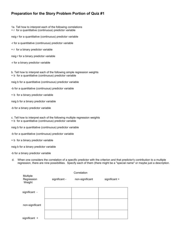
Preparation for the Story Problem Portion of Quiz #1
1a. Tell how to interpret each of the following correlations
+ r for a quantitative (continuous) predictor variable
nsig r for a quantitative (continuous) predictor variable
-r for a quantitative (continuous) predictor variable
+ r for a binary predictor variable
nsig r for a binary predictor variable
-r for a binary predictor variable
b. Tell how to interpret each of the following simple regression weights
+ b for a quantitative (continuous) predictor variable
nsig b for a quantitative (continuous) predictor variable
-b for a quantitative (continuous) predictor variable
+ b for a binary predictor variable
nsig b for a binary predictor variable
-b for a binary predictor variable
c. Tell how to interpret each of the following multiple regression weights
+ b for a quantitative (continuous) predictor variable
nsig b for a quantitative (continuous) predictor variable
-b for a quantitative (continuous) predictor variable
+ b for a binary predictor variable
nsig b for a binary predictor variable
-b for a binary predictor variable
d.
When one considers the correlation of a specific predictor with the criterion and that predictor's contribution to a multiple
regression, there are nine possibilities. Specify each of them (there might be a "special name" or maybe just a description.
Correlation
Multiple
Regression
Weight
significant -
non-significant
significant +
significant -
non-significant
significant +
Answers
1a. interpreting correlations
quant predictors
+r direct relationship -- those with higher scores on the predictor tend to have higher scores on the criterion (and vice versa)
nsig r no reliable relationship between pred and crit -- knowing value of one tells you nothing about value of the other
-r indirect relationship -- those with higher scores on the predictor tend to have lower scores on the criterion (and vice versa)
binary predictors
+r group with higher coded value has higher mean score on the criterion (and vice versa)
nsig r no reliable mean difference on the criterion between the groups
-r group with the higher coded value has lower mean score on the criterion (and vice versa)
b. interpreting simple regression weights
quant predictors
+b direct relationship -- each 1-point increase in the predictor is expected to be associated with an increase in the predicted
criterion score equal to "b"
nsig b no reliable prediction about the change in the predicted criterion score based on changes in that predictor,
-b indirect relationship -- each 1-point increase in the predictor is expected to be associated with an decrease in the predicted
criterion score equal to "b"
binary predictors
+b group with higher coded value had a mean on the criterion score "b" higher than the group with the lower coded score
nsig b no reliable mean difference on the criterion between the groups
-b group with higher coded value had a mean on the criterion score "b" lower than the group with the lower coded score
c. interpreting multiple regression weights
quant predictors
+b direct relationship -- each 1-point increase in the predictor is expected to be associated with an increase in the predicted
criterion score equal to "b", if the values of the other predictors are held constant (controlled for) (and vice versa)
nsig b no reliable prediction about the change in the predicted criterion score based on changes in that predictor, ", if the values of
the other predictors are held constant (controlled for) (and vice versa)
-b indirect relationship -- each 1-point increase in the predictor is expected to be associated with an decrease in the predicted
criterion score equal to "b", if the values of the other predictors are held constant (controlled for) (and vice versa)
binary predictors
+b group with higher coded value had a mean on the criterion score "b" higher than the group with the lower coded score, if the
values of the other predictors are held constant (controlled for) (and vice versa)
nsig b no reliable mean difference on the criterion between the groups, if the
values of the other predictors are held constant
(controlled for)
-b group with higher coded value had a mean on the criterion score "b" lower than the group with the lower coded score, if the values
of the other predictors are held constant (controlled for) (and vice versa)
Considering correlations and regression weights
Correlation
Multiple
Regression
Weight
significant -
significant -
***
non-significant
^^^
significant +
!!!
non-significant
significant +
!!!
boring variable
!!!
!!!
^^^
***
*** good correlate & direct contributor ^^^ good correlate, but collinear with other predictors !!! Supressor variable
Practice with collinearity, etc. –this won’t be on the quiz, but may help you understand other things better!!
Answer the following questions based on the information in the correlation matrix -- pay careful attention to how the answers change
and don't change as the correlations change!
Here are the correlations from a sample of therapy patients -- wellness is the criterion variable.
Wellness
Well
Age
Initial
Prior
Current
1.00
.42
.38
.41
.39
Age
.42
1.00
.40
.61
.23
Initial
Amount
Wellness Prior
Therapy
.38
.40
1.00
.15
-.63
.41
.61
.15
1.00
.36
Number of
Current
Sessions
.39
.23
.23
-.63
1.00
a. What is the best single predictor of wellness ?
b. What predictor would you add to the variable you chose in "a" to produce the largest increase in R²? Explain your answer.
c.
Reconsider the information in the correlation matrix. Is the two-predictor model you chose in "a & b" likely to be best 2-predictor
model available from these variables? If not, what do you think will likely be the best two-predictor model? Explain your answer.
Initial Amount Number of
Wellness Age Wellness Prior Current
Therapy Sessions
Well
Age
Initial
Prior
Current
1.00
.40
.38
.41
.39
.40 .38
.41
1.00 .40
.61
.40 1.00 .15
.61 .15 1.00
.33 .33 -.63
.39
.33
.33
-.63
1.00
d.
What is the best single predictor of wellness ?
e.
What predictor would you add to the variable you chose in "a" to produce the largest increase in R²? Explain your answer.
f.
Reconsider the information in the correlation matrix. Is the two-predictor model you chose in "a & b" likely to be best 2-predictor
model available from these variables? If not, what do you think will likely be the best two-predictor model?
Initial Amount Number of
Wellness Age Wellness Prior
Current
Therapy Sessions
Well 1.00 .42 .18 .21
Age
.42 1.00 .2 0 .21
Initial .18
.20 1.00 .15
Prior
.21
.21 .15 1.00
Current .39
.23 .13 .16
.39
.23
.13
.16
1.00
g.
What is the best single predictor of wellness ?
h.
What predictor would you add to the variable you chose in "a" to produce the largest increase in R²?
i.
Reconsider the information in the correlation matrix. Is the two-predictor model you chose in "a & b" likely to be best 2-predictor
model available from these variables? If not, what do you think will likely be the best two-predictor model?
ANSWERS to Practice with Collinearity
a.
Age has the highest bivariate correlation -- so is the best single predictor
b.
The other predictors are similarly correlated with the criterion, but #current has the lowest collinearity with age, and so will lead to
the largest increase in R² if added to age
c.
Again, all the predictors are similarly correlated with the criterion, so the answer to this question is going to hinge on the
collinearities. Consider initial and amount prior, which are nearly as correlated with the criterion as are age and #current, but which
have a lower collinearity with each other (suggesting they will have a higher 2-predictor R²)
d.
Amount of prior therapy has the highest correlation -- so it is the best single predictor
e.
The rest of the predictors are about equally correlated with the criterion, but initial wellness has the lowest collinearity with amount
of prior therapy -- so it will lead to the largest increase in R² if added to amount of prior therapy
f.
The predictors all have about the same correlation with the criterion, but initial wellness and amount of prior therapy have the
lowest collinearity (by far) -- so these two probably will lead to the best two-predictor model
g.
Age is the best single predictor
h.
The other three predictors have about the same collinearity with age --however Number of current sessions has a much larger
correlation with the criterion, and so will lead to the largest in R² if added to age.
i.
Age and Number of current sessions have higher simple correlations with the criterion than the other two predictors. Also, the
collinearity among pairs of the other predictors are not much lower than between age and number of current sessions, so it is likely
that age and number of current sessions will produce the best two-predictor model.
Correlation, Bivariate & Multivariate Regression -- Practice #1
Correlations
RATING2
Pears on Correlation
Sig. (2-tailed)
N
AGE
.357
.035
120
GENDER
.013
.891
120
SALARY
.826
.000
120
NFRNDS
-.354
.036
120
a. Should I be concerned about the statistical power involved in the gender correlation? Carefully explain your
answer.
b. Should I be concerned about the statistical power involved in the age? Carefully explain your answer
Correlations
RATING2
Pears on Correlation
Sig. (2-tailed)
N
AGE
.357
.035
120
GENDER
.013
.891
120
Model Summary
SALARY
.826
.000
120
NFRNDS
-.354
.036
120
Model
1
Std. Error of
the Es timate
2.28317
a. Predictors : (Cons tant), NFRNDS, SALARY, AGE,
GENDER
a. What are the viable individual predictors?
ANOVAb
Model
1
b.
Adjus ted
R Square
.674
R
R Square
.828 a
.685
Interpret the simple correlation of age.
Regress ion
Res idual
Total
Sum of
Squares
1304.528
599.481
1904.009
df
4
115
119
Mean Square
326.132
5.213
F
62.563
Sig.
.000 a
a. Predictors : (Cons tant), NFRNDS, SALARY, AGE, GENDER
b. Dependent Variable: RATING4
c.
d.
e.
Coefficientsa
Interpret the simple correlation of gender.
Does the model work? What did you look at to decide?
Model
1
How well does the model work?
(Cons tant)
AGE
GENDER
SALARY
NFRNDS
Uns tandardized
Coefficients
Std.
B
Error
.352
1.704
.027
.042
10.244
.425
.030
.000
-.402
.074
a. Dependent Variable: RATING4
f.
Which predictors contribute to the model? What did you look at to decide?
g.
Would the model “do as well” if age were dropped from the model? Explain your answer.
h.
Would the model “do as well” if salary were dropped from the model? Explain your answer.
i.
That is the most likely reason that age is not contributing to the model?
j.
Interpret the multiple regression weight for gender.
k.
Interpret the multiple regression weight for number of friends
l.
Tell the suppressor variables ( if there are any).
Standardized
Coefficients
Beta
.034
.030
.826
.001
t
.206
.643
24.57
15.74
5.343
Sig.
.837
.522
.001
.003
.040
Answers for Correlation, Bivariate & Multivariate Regression -- Practice #1
a. Should I be concerned about the statistical power involved in the gender correlation? Carefully explain your
answer.
Since the effect size ( r ) was so small ( < .10) the most likely reason for retaining H0: is that the population effect
is very small, not that there’s a sample size/power problem.
b. Should I be concerned about the statistical power involved in the age? Carefully explain your answer.
No! We rejected H0: (p < .05) and so, by definition, we had enough power for this analysis (which is not to say
that we should automatically use N=120 for a replication study. An a priori power analysis should be done.)
a. What are the viable individual predictors?
Age, Salary & Nfrnds – have significant correlations
b.
Interpret the simple correlation of age.
Older participants tend to give higher liking ratings.
c.
Interpret the simple correlation of gender.
There no linear relationship between gender and rating.
d.
Does the model work? What did you look at to decide?
Yes! ANOVA test of R² is significant
e.
How well does the model work?
R² = .685 which is a “strong” model
f.
Which predictors contribute to the model? What did you look at to decide?
Gender, Salary and Nfrnds -- all have significant p=-values of the t-test that b=0
g.
Would the model “do as well” if age were dropped from the model? Explain your answer.
Age does not contribute, so the model would do “as well” if it were dropped. R² would drop, but not significantly.
h.
Would the model “do as well” if salary were dropped from the model? Explain your answer.
Salary does contribute, so the model would not do “as well” if it were dropped. R² would drop significantly.
i.
What is the most likely reason that age is not contributing to the model?
Age is significantly correlated with the criterion, so the most likely reason it isn’t contributing to the multiple
regression model is that it is collinear with one or more of the other variables in the model.
j.
Interpret the multiple regression weight for gender.
Females (with the higher code) gave a mean liking rating 10.244 higher than males, after controlling for the other
variables in the model. That mean difference is statistically significant.
k.
Interpret the multiple regression weight for number of friends
With increase of one friend the expected rating goes down by .402, after controlling for the other variables in the
model.
l.
Tell the suppressor variables ( if there are any).
Gender is a suppressor – it is not correlated but has a significant contribution to the multivariate model.
Correlation, Bivariate & Multivariate Regression -- Practice #2
Correlations
NUMLOS
T
Pears on Correlation
Sig. (2-tailed)
N
MOMA
GE
.035
.834
80
DADAGE
.292
.030
80
MOMRA
TE
-.130
.214
80
DADRAT
E
.431
.036
80
a. Should I be concerned about the statistical power involved in the momrate correlation? Carefully explain your answer.
b. Should I be concerned about the statistical power involved in the dadrate correlation? Carefully explain your answer.
An additional analysis of the survey data was designed to examine whether we could predict the number of times parents had “lost” a
child in a public place for at least 5 minutes (NUMLOST) from the parent’s age (MOMAGE & DADAGE, and their ratings of concern
about children playing in public (MOMRATE & DADRATE).
Here’ s the SPSS output from the simple correlations and the multiple regression analysis.
Correlations
NUMLOS
T
Pears on Correlation
Sig. (2-tailed)
N
MOMA
GE
.035
.834
80
Model Summary
DADAGE
.292
.030
80
MOMRA
TE
-.130
.214
80
DADRAT
E
.431
.036
80
Model
1
R
R Square
.456 a
.208
ANOVAb
Model
1
Interpret the simple correlation of MOMAGE.
Std. Error of
the Es timate
1.18317
a.
a. What are the viable individual predictors?
b.
Adjus ted
R Square
.197
Regress ion
Res idual
Total
Sum of
Squares
1304.528
599.481
1904.009
df
4
115
119
Mean Square
326.132
5.213
F
62.563
Sig.
.000 a
a. Predictors : (Cons tant), NFRNDS, SALARY, AGE, GENDER
b. Dependent Variable: RATING4
c.
Interpret the simple correlation of DADRATE.
d.
Does the model work? What did you look at to decide?
e.
Coefficientsa
Model
1
How well does the model work?
Uns tand
ardi zed
Coeffi ci
ents
B
(Cons tant)
MOMAGE
DADAGE
MOMRATE
DADRATE
Standardized
Coeffi cients
.352
.827
.424
-.499
.986
a. Dependent Variable: RATING4
f.
Which predictors contribute to the model? What did you look at to decide?
g.
Would the model “do as well” if DADAGE were dropped from the model? Explain your answer.
h.
Would the model “do as well” if DADRATE were dropped from the model? Explain your answer.
i.
What is the most likely reason that MOMAGE is not contributing to the model?
j.
Interpret the multiple regression weight for DADAGE.
k.
Interpret the multiple regression weight for MOMRATE
l.
Tell the suppressor variables ( if there are any).
Beta
.134
.030
.826
.001
Sig.
.837
.522
.001
.003
.098
Answers for Correlation, Bivariate & Multivariate Regression -- Practice #2
a. Should I be concerned about the statistical power involved in the momrate correlation? Carefully explain your answer.
Informal Answer: This effect is large enough that, if it were significant, we would likely be interested in the effect,
so retaining the null is likely to be a type II error, produced by the small sample size.
b. Should I be concerned about the statistical power involved in the dadrate correlation? Carefully explain your answer.
No! We “must have had enough power” because we rejected H0: (p < .05)
Here’ s the SPSS output from the simple correlations and the multiple regression analysis.
a. What are the viable individual predictors?
DADAGE & DADRATE p-value of correlations
b.
Interpret the simple correlation of MOMAGE.
c. MOMAGE
Interpret theisn’t
simple
correlated
correlationwith
of DADRATE.
NUMLOST
Dads with more concern tend to “lose” more children
d.
Does the model work? What did you look at to decide?
Yes – p-value of ANOVA
e.
How well does the model work?
f.
Which predictors contribute to the model? What did you look at to decide?
R² = .208
DADAGE & MOMRATE
g.
Would the model “do as well” if DADAGE were dropped from the model? Explain your answer.
No – DADAGE is contributing to the model, so dropping it would lead to a significant drop in R²
h.
Would the model “do as well” if DADRATE were dropped from the model? Explain your answer.
Yes – DADRATE is not contributing to the model, so dropping it will not lead to a significant drop in R²
i.
What is the most likely reason that MOMAGE is not contributing to the model?
The most likely reason is that MOMAGE is not correlated with the criterion variable
j.
Interpret the multiple regression weight for DADAGE.
For each 1-year increase in Dad’s age the expected number of lost children increases by .424, after controlling
for the other variables in the model
k.
Interpret the multiple regression weight for MOMRATE
For each 1-unit increase in Mom’s concern rate the expected number of lost children decreases by .499, after
controlling for the other variables in the model
l. Tell the suppressor variables ( if there are any).
MOMRATE is a suppressor – not correlated, but contributes to the multivariate model
More Practice w/ bivariate & multivariate
Here's a set of correlations and a full-model regression with "Therapeutic Outcome" (larger scores are "better") for "Type of Therapy"
(1=conventional 2=experimental).
Predictor ==>
Age
correlation
(p-value)
reg. weight
(p-value)
.42
(.03)
-3.21
(.01)
Initial
Wellness
.38
(.04)
2.21
(.89)
Amount
Prior
Therapy
-.43
(.03)
Number of
Current
Sessions
.18
(.21)
-1.89
(.14)
.512
(.04)
a. Based on the simple correlations, which are viable single predictors?
b. How would you interpret the correlation of the following predictors and the criterion variable?
Age
Amount of Prior Therapy
Type of Therapy
c. Which predictors are contributing to the full model?
d. How would you interpret the multiple regression weight of the following predictors?
Age
Initial Wellness
Number of Current sessions
Type of Therapy
e. What is the most likely reason that Initial Wellness is not contributing to the full model?
f. What is the most likely reason that Type of Therapy is contributing to the full model?
g. Any suppressor variables? How would you NOT want to interpret the regression weight of that variable?
Type of
Therapy
.45
(.03)
8.24
(.04)
Still More Practice w/ bivariate & multivariate
GENDER (1=male, 2=female)
SCTYP (school type; 2=public 1=private) SES (1 = low, 2 = mid)
The criterion is performance on a standardized "senior examination" which must be passed to graduate.
a.
Predictor ==>
SCTYP
GENDER
SES
Correlation
(p-value)
-.18
(.04)
.14
(.20)
.58
(.01)
reg. weight
(p-value)
-.821
(.01)
.873
(.04)
.005
(.89)
RDG
.61
(.01)
.343
(.02)
WRTG
MATH
SCI
ABSENCES
.06
(.62)
.13
(.44)
.51
(.01)
-.31
(.04)
.049
(.71)
.0001
(.97)
.434
(.01)
-.121
(.132)
Circle the correlations of the viable single predictors?
b. Circle the regression weights of those predictors that are contributing to the full model?
c.
Put a square around any predictors that are not contributing to the full model "probably because they are not sufficiently strongly
related to the criterion variable."
d.
Put a triangle around any predictors that are not contributing to the full model "probably because they are collinear with one or
more of the other variables."
e.
List the names of any "suppressor variables" below.
f.
Tell the meaning of the SCTYP correlation in words.
g.
Tell the meaning of the SCI correlation in words.
h.
Tell the meaning of the GENDER correlation in words.
i.
Tell the meaning of the ABSENCES correlation in words.
j.
Based on the weights from the full regression model, if my estimated senior exam score were 85, but I just re-took
READING test and scored 10 points higher ! What would be the new estimate of my senior exam score?
Answers for More Practice w/ bivariate & multivariate
a. Age, Initial Wellness, Amount of Prior Therapy & Type of Therapy -- all p < .05
b. Age -- older patients tend to have higher Therapeutic Outcome scores.
Amount of Prior Therapy -- those with less prior therapy tend to have higher Therapeutic Outcome scores
Number of Current Sessions -- no reliable bivariate relationship
Type of Therapy -- those receiving the experimental therapy has a higher average Therapeutic Outcome score
c. Age, Number of Current Sessions, Type of Therapy
d. Age -- a 1-year increase in age is associated with a 3.21 decrease in predicted Therapeutic Outcome score, holding scores on
all other predictors constant
Initial Wellness -- after holding scores on all other predictors constant, there is no reliable expected change in Therapeutic
Outcome score associated with differences in Initial wellness
Number of Current Sessions -- each additional current session is associated with a .512 increase in predicted Therapeutic
Outcome score, holding scores on all other predictors constant
Type of Therapy -- Those receiving the experimental treatment have mean Therapeutic Outcome score 8.24 higher than those in
the conventional treatment group, holding constant (controlling for) scores on all the other predictors constant
e. It is collinear with one or more of the other variables in the multiple regression model
f. It is correlated with the criterion and is not strongly collinear with the other variables in the multiple regression model
g. Age (+r but -b) and Number of Current Sessions (0r but +b). Don't interpret the regression
weight as telling you the direction
and/or strength of the bivariate relationship between that
predictor and the criterion
Answers for Still More Practice w/ bivariate & multivariate
a. viable single predictors include sctypm ses, rdg, sci & absences
b. regression contributors included sctyp, gender, rdg & sci
c.
"not correlated" non-contributors included wrtg and math
d. "collinear" non-contributors included ses & absences
e. gender is a suppressor
f.
the "-" correlation indicates that private school students (with the smaller code values) tend to have higher mean exam
scores than public school students (with the larger code values)
g. those with higher math scores tend to have higher exam scores
h. we would interpret this "non-significant" correlation to mean there is no linear relationship between the variables -that's what H0: testing means (a couple acknowledged the non-significance and then interpreted the correlation,
based on the idea the effect size wasn't trivial -- that's OK, but may get punished in research reports!
i.
the "-" correlation indicates that those with fewer absences tend to have higher exam scores
j.
A multiple regression weight tells the expected change in the criterion for a 1-unit change in that predictor, if the
values of all other predictors are held constant, so 85 + (10 * .343) = 88.43. I was delighted in the number
of folks
who got this !!!
What Next & What If (and a few conceptual things) Practice #1
Consider these output from a step in an algorithm-driven modeling (criterion = wellness) and answer the questions.
Variables in Equation
variable
Weight
Gender
Pred2
Pred5
b
3.26
14.73
.02
123.44
p (of t)
Variables not in Equation
variable
.43
.06
.02
.04
a. if this were a forward selection -- what would happen next?
b. if this were a backward selection -- what would happen next?
Pred4
Pred1
Pred3
Age
partial
.48
.51
.46
.15
p of t (if entered)
.01
.02
.01
.53
Would the R² change significantly?
Would the R² change significantly?
c. if this were a forward stepwise selection -- what would happen next?
Would the R² change significantly?
d. What would happen to the R² if I added Pred3 to the model? Explain your answer.
e. What would happen to the R² if I added Age to the model? Explain your answer.
f. What would happen to the R² if I deleted weight from the model? Explain your answer.
g. What would happen to the R² if I deleted Pred2 from the model? Explain your answer.
h. What would happen if I deleted both Weight and Gender from the model? Explain your answer.
i. What would happen to the R² if I deleted both Pred2 and Pred5 from the model? Explain your answer.
j. What would happen to the R² if I deleted both Weight and Pred2 from the model? Explain your answer.
What Next & What If (and a few conceptual things) Practice #2
1.
Consider these output from a step in an algorithm-driven modeling and answer the questions.
Variables in Equation
variable
b
Age
.21
Gender
4.22
Pred1
1.02
Pred4
123.44
constant 9.0
Variables not in Equation
p (of t)
variable
.43
.04
.02
.01
.02
Pred 2
Pred 3
Pred 5
a. if this were a forward selection -- what would happen next?
partial
.01
.12
.08
p of t (if entered)
.98
.01
.43
Would the R-square change significantly?
b. if this were a backward selection -- what would happen next?
c. if this were a stepwise selection -- what would happen next?
Would the R-square change significantly?
Would the R-square change significantly?
Consider these output from a step in an algorithm-driven modeling (criterion = wellness) and answer the questions.
Variables in Equation
variable
b
p (of t)
Weight
3.26
.43
Gender
14.73
.06
Pred2
.02
.02
Pred5
123.44
.04
Variables not in Equation
variable
partial
p of t (if entered)
Pred4
.48
.01
Pred1
.51
.02
Pred3
.46
.01
Age
.15
.53
d.
if this were a forward selection -- what would happen next?
Would the R change significantly?
e.
if this were a backward selection -- what would happen next?
f.
if this were a forward stepwise selection -- what would happen next?
g.
What would happen to the R if I added Pred3 to the model? Explain your answer.
h.
If I dropped Pred5, Pred2 and Gender from the model, would the R be significantly larger than 0? Explain your
answer.
i.
What would happen to the R if I swapped (replaced with, substituted, whatever) Pred1 for Weight in this model?
(Hint: you CAN predict the result of this from the available data! But how?)
Would the R change significantly?
Would the R change significantly?
Answers for What Next & What If (and a few conceptual things) Practice #1
Consider these output from a step in an algorithm-driven modeling (criterion = wellness) and answer the questions.
a. Add pred1 -- has highest partial of the viable candidates for inclusion. R² will increase significantly
b. Toss weight -- has largest p-value of the viable candidates for exclusion
c. same as "b"
d. Adding a significant (contributing) predictor to the model would increase R² significantly
e. Adding a non-significant (non-contributing) predictor to the model would increase R² numerically, but not significantly
f. Dropping a non-significant (non-contributing) predictor to the model would decrease R² numerically, but not significantly
g. Dropping a significant (ontributing) predictor to the model would decrease R² significantly
h. Neither predictor is contributing and we could drop either one without r² decreasing significantly. It is unlikely that dropping both
will lead to a decrease in R². Why? Of the two, the larger R² decrease isn't significant, and so the average R² difference
from dropping the two of them is unlikely to be significant
i. Because both are contributing, and dropping either would lead to a significant decrease in R², it is likely that dropping both would
lead to significant average drop in R²
j. This is the "iffy one" -- dropping one would lead to a decrease, dropping the oher wouldn't, and we have no way of estimating the
result of the "average drop" -- so for this one we should plead "I don't know" and do the nested model comparison test.
Answers for What Next & What If (and a few conceptual things) Practice #2
a.
Add Pred 3. Yes, the Rsqr will increase significantly, because we will be adding a contributing predictor.
b.
Drop Age. No, the Rsqr will not drop significantly, because we are eliminating a noncontributing predictor.
c.
Same as "b"
d.
We would be adding another predictor, if there is one that would increase R² significantly. Pred4, Pred1 and Pred3 are all
candidates, because each would have a contribution if it were added to the existing model (as shown by the significant p or t). Of
these, Pred1 has the highest partial (and so part) correlation, and so is the one which would increase R² the most -- add Pred1.
The R² will go up significantly, because the added predictor will contribute to the model.
e.
We would be dropping another predictor, if there is one to drop that will not lead to a significant drop in variance
accounted for
(i.e., if there is a non-contributing predictor). Weight and gender are both candidates for exclusion, since neither of them is
contributing to the model. Of these, weight is less likely to be contributing, so we would drop it. There will be no significant drop in
variance accounted for, because we are dropping a non-contributing predictor.
f.
Forward stepwise checks that all included predictors are contributing before adding any additional predictors. In this case, the next
step would be the same as the next step of the backward procedure.
g.
R² would increase significantly, because we would be adding a contributing predictor.
h.
Yes, that would leave weight, which was the first predictor into the model (or at least the sole predictor at one point), and so must
have had a significant simple correlation with the criterion.
i.
Dropping weight would not lead to a significant drop in R², adding Pred1 would lead to a significant increase in R², so the
combined effect would be a significant increase in R².
Identifying Models, Model Comparisons & Significance Tests – Practice #1
This form of practice is a bit different from what is in the Demo and what will appear on the
Quiz. This asks you to “pick out” the question/hypothesis, as well as label it…
The overall purpose of the study is to examine relationships between school grades, prior work experience and
interview process scores to predict job performance (jp; derived from work performance during the 1 st six months of work).
Here are the predictors..








high school grades (hsg)
# school absences (has)
food service classes in high school (hsvs)
# prior jobs (jobs)
why left last job (quit or fired; last)
how long on prior job (long)
interview score (int)
interview performance score (perf)
My colleagues and I have several questions and hypotheses!
Are high school grades related to job performance. Is number or prior jobs an important intermediate variable to
understanding this relationship? What about after we control both for number of prior jobs, or both number of prior jobs
and whether or not they have had food service classes? Will the model with all these predictors help us identify better
workers? Do high school grades have both direct and indirect effects upon job performance? Will dropping the interview
performance test hurt how well we can predict? What about if we drop both interview measures? I think that high school
information will predict worker performance better than information from the interview and as well as using all the
predictors together. What is the best predictor of job performance among the high school variables, and is it a better
predictor than the interview score? Not everyone has had a job before, does the interview score work better for those
who have or those who haven't had a job before. For that matter, do the combination of interview score and interview
performance score and number of prior jobs work better for those who have or those who haven't had a job before. And
are different predictors most important for the model in these two populations? I think that when we consider the
relationship between interview score and job performance we need to control interview scores for whether or not they've
had a food service class in high school -- you know they practice interviewing in those classes.
Answers for Identifying Models, Model Comparisons & Significance Tests – Practice #1
Are high school grades related to job performance.
Simple correlation, direct p-value
Is number or prior jobs an important intermediate variable to understanding this relationship?
Mediation analysis, comparison of r & beta
What about after we control both for number of prior jobs,
Partial correlation, direct p-value
or both number of prior jobs and whether or not they have had food service classes?
Multiple partial correlations, direct p-value
Will the model with all these predictors help us identify better workers?
Multiple regression, R-sq F-test
Do high school grades have both direct and indirect effects upon job performance?
Path Analysis, analysis of b and Beta weights
Will dropping the interview performance test hurt how well we can predict?
Nested model comparison, Rsq-change F-test
What about if we drop both interview measures?
Nested model comparison, Rsq-change F-test
I think that high school information will predict worker performance better than information from the interview
Comparing correlated correlations, Steiger’s Z
and as well as using all the predictors together.
Comparing non-nested models, Steiger’s Z
What is the best predictor of job performance among the high school variables,
Comparing correlated correlations, Steiger’s Z
and is it a better predictor than the interview score?
Comparing correlated correlations, Steiger’s Z
Not everyone has had a job before, does the interview score work better for those who have or those who haven't had a
job before.
Comparing a correlation across populations, Fisher’s Z
For that matter, do the combination of interview score and interview performance score and number of prior jobs work
better for those who have or those who haven't had a job before.
Comparing a regression model across populations, Fisher’s Z
And are different predictors most important for the model in these two populations?
Comparing a regression model across populations, Steiger’s Z
I think that when we consider the relationship between interview score and job performance we need to control interview
scores for whether or not they've had a food service class in high school -- you know they practice interviewing in those
classes.
Semi partial correlation, direct p-value
Answers for Identifying Models, Model Comparisons & Significance Tests – Practice #2
In effort to evaluate what makes some print advertisements successful and others not, we generated several ads that
had various combinations of the following attributes. When collecting the data each participant viewed one ad, rated how
much they thought it would "influence their opinion of the product" (inop) and complete a questionnaire involving some
self-descriptive questions. The predictor variable set included…






ad size (size)
color or black & white ( col)
people in ad (peo)
rater's age (age)
rater's gender (sex)
rater's familiarity with the product (fam)
Once we include the ad variables I'm not sure that the rater variables will add anything. Except it might be that adding
just rater familiarity with the product to the ad variables will help. A related question to ask is if ad attributes are more
important than viewer attributes, and whether viewer attributes have direct effects or if they are indirect through ad
attributes. Either way, I think that the way the ad variables relate to the criterion will be different for males and females,
and they will predict far better for males. Well, I think that size and color will correlate with ability to influence equally for
males and females, but that people being in the ad is more correlated with ability to influence for females than for males. I
think that whether ads use color or black & white is related to their ability to influence opinion (even if you control for
gender or gender and age) and that this is a more important predictor than the ad size or whether or not people are in the
ad. What I really think is going on here is that color versus black & white adds is an important intermediate variable when
understanding the relationship between gender and the ad’s ability to influence opinion.
Answers for Identifying Models, Model Comparisons & Significance Tests – Practice #2
Once we include the ad variables I'm not sure that the rater variables will add anything.
Nested model comparison, Rsq-change F-test
Except it might be that adding just rater familiarity with the product to the ad variables will help.
Nested model comparison, Rsq-change F-test
A related question to ask is if ad attributes are more important than viewer attributes.
Non-nested model comparison, Steiger’s Z
, and whether viewer attributes have direct effects or if they are indirect through ad attributes
Path analysis, t-tests of b & Beta weights
Either way, I think that the way the ad variables relate to the criterion will be different for males and females.
Comparing a model across populations, Steiger’s Z
and they will predict far better for males.
Comparing a model across populations, Fisher’s Z
Well, I think that size and color will correlate with ability to influence equally for males and females,
Comparing correlations across populations (not comparing models because it specifically says “correlate”), Fisher’s Z
but that people being in the ad is more correlated with ability to influence for females than for males.
Comparing correlations across populations, Fisher’s Z
I think that whether ads use color or black & white is related to their ability to influence opinion
Simple correlation, direct p-values
(even if you control for gender
Partial correlation, direct p-values
or gender and age)
Multiple partial correlation, direct p-values
and that this is a more important predictor than the ad size
Comparing correlated correlations, Steiger’s Z
or whether or not people are in the ad.
Comparing correlated correlations, Steiger’s Z
What I really think is going on here is that color versus black & white adds is an important intermediate variable when
understanding the relationship between gender and the ad’s ability to influence opinion.
Mediation analysis, comparing r & Beta weights