BMVC abstract template
advertisement
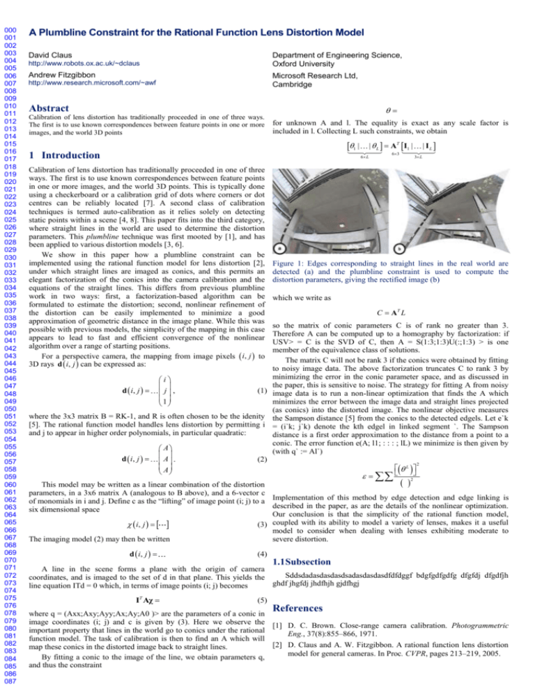
000 001 002 003 004 005 006 007 008 009 010 011 012 013 014 015 016 017 018 019 020 021 022 023 024 025 026 027 028 029 030 031 032 033 034 035 036 037 038 039 040 041 042 043 044 045 046 047 048 049 050 051 052 053 054 055 056 057 058 059 060 061 062 063 064 065 066 067 068 069 070 071 072 073 074 075 076 078 079 080 081 082 083 084 085 086 087 A Plumbline Constraint for the Rational Function Lens Distortion Model David Claus Department of Engineering Science, Oxford University http://www.robots.ox.ac.uk/~dclaus Andrew Fitzgibbon Microsoft Research Ltd, Cambridge http://www.research.microsoft.com/~awf Abstract Calibration of lens distortion has traditionally proceeded in one of three ways. The first is to use known correspondences between feature points in one or more images, and the world 3D points for unknown A and l. The equality is exact as any scale factor is included in l. Collecting L such constraints, we obtain 1 | 1 Introduction | L AT I1 | 6 L Calibration of lens distortion has traditionally proceeded in one of three ways. The first is to use known correspondences between feature points in one or more images, and the world 3D points. This is typically done using a checkerboard or a calibration grid of dots where corners or dot centres can be reliably located [7]. A second class of calibration techniques is termed auto-calibration as it relies solely on detecting static points within a scene [4, 8]. This paper fits into the third category, where straight lines in the world are used to determine the distortion parameters. This plumbline technique was first mooted by [1], and has been applied to various distortion models [3, 6]. We show in this paper how a plumbline constraint can be implemented using the rational function model for lens distortion [2], under which straight lines are imaged as conics, and this permits an elegant factorization of the conics into the camera calibration and the equations of the straight lines. This differs from previous plumbline work in two ways: first, a factorization-based algorithm can be formulated to estimate the distortion; second, nonlinear refinement of the distortion can be easily implemented to minimize a good approximation of geometric distance in the image plane. While this was possible with previous models, the simplicity of the mapping in this case appears to lead to fast and efficient convergence of the nonlinear algorithm over a range of starting positions. For a perspective camera, the mapping from image pixels i, j to 3D rays d i, j can be expressed as: 6 3 | IL 3 L Figure 1: Edges corresponding to straight lines in the real world are detected (a) and the plumbline constraint is used to compute the distortion parameters, giving the rectified image (b) which we write as C AT L so the matrix of conic parameters C is of rank no greater than 3. Therefore A can be computed up to a homography by factorization: if USV> = C is the SVD of C, then A = S(1:3;1:3)U(:;1:3) > is one member of the equivalence class of solutions. The matrix C will not be rank 3 if the conics were obtained by fitting to noisy image data. The above factorization truncates C to rank 3 by minimizing the error in the conic parameter space, and as discussed in i the paper, this is sensitive to noise. The strategy for fitting A from noisy d i, j j , (1) image data is to run a non-linear optimization that finds the A which 1 minimizes the error between the image data and straight lines projected (as conics) into the distorted image. The nonlinear objective measures where the 3x3 matrix B = RK-1, and R is often chosen to be the idenity the Sampson distance [5] from the conics to the detected edgels. Let e`k [5]. The rational function model handles lens distortion by permitting i = (i`k; j`k) denote the kth edgel in linked segment `. The Sampson and j to appear in higher order polynomials, in particular quadratic: distance is a first order approximation to the distance from a point to a conic. The error function e(A; l1; : : : ; lL) we minimize is then given by A (with q` := Al`) d i, j A . (2) 2 A L 2 This model may be written as a linear combination of the distortion parameters, in a 3x6 matrix A (analogous to B above), and a 6-vector c of monomials in i and j. Define c as the “lifting” of image point (i; j) to a Implementation of this method by edge detection and edge linking is described in the paper, as are the details of the nonlinear optimization. six dimensional space Our conclusion is that the simplicity of the rational function model, i, j (3) coupled with its ability to model a variety of lenses, makes it a useful model to consider when dealing with lenses exhibiting moderate to severe distortion. The imaging model (2) may then be written d i, j (4) 1.1 Subsection A line in the scene forms a plane with the origin of camera Sddsdadasdasdasdsadasdasdasdfdfdggf bdgfgdfgdfg dfgfdj dfgdfjh coordinates, and is imaged to the set of d in that plane. This yields the ghdf jhgfdj jhdfhjh gjdfhgj line equation ITd = 0 which, in terms of image points (i; j) becomes IT Aχ (5) References where q = (Axx;Axy;Ayy;Ax;Ay;A0 )> are the parameters of a conic in image coordinates (i; j) and c is given by (3). Here we observe the [1] D. C. Brown. Close-range camera calibration. Photogrammetric important property that lines in the world go to conics under the rational Eng., 37(8):855–866, 1971. function model. The task of calibration is then to find an A which will [2] D. Claus and A. W. Fitzgibbon. A rational function lens distortion map these conics in the distorted image back to straight lines. model for general cameras. In Proc. CVPR, pages 213–219, 2005. By fitting a conic to the image of the line, we obtain parameters q, and thus the constraint 2 BUCH, ORWELL, VELASTIN: 3DHOG FOR CLASSIFICATION OF ROAD USERS [3] F. Devernay and O. Faugeras. Straight lines have to be straight. MVA, 13:14–24, 2001. [4] A. W. Fitzgibbon. Simultaneous linear estimation of multiple view geometry and lens distortion. In Proc. CVPR, 2001. [5] R. I. Hartley and A. Zisserman. Multiple View Geometry in Computer Vision. Cambridge University Press, ISBN: 0521623049, 2000. [6] R. Swaminathan and S. Nayar. Nonmetric calibration of wide-angle lenses and polycameras. IEEE T-PAMI, 22(10):1172–1178, 2000. [7] Y. R. Tsai. An efficient and accurate camera calibration technique for 3D machine vision. In Proc. CVPR, 1986. [8] Z. Zhang. On the epipolar geometry between two images with lens distortion. In Proc. ICPR, pages 407–411, 1996.
