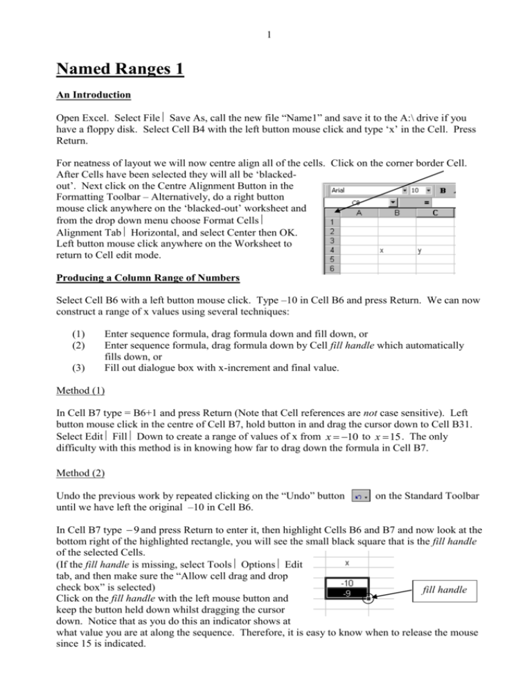
1
Named Ranges 1
An Introduction
Open Excel. Select File  Save As, call the new file “Name1” and save it to the A:\ drive if you
have a floppy disk. Select Cell B4 with the left button mouse click and type ‘x’ in the Cell. Press
Return.
For neatness of layout we will now centre align all of the cells. Click on the corner border Cell.
After Cells have been selected they will all be ‘blackedout’. Next click on the Centre Alignment Button in the
Formatting Toolbar – Alternatively, do a right button
mouse click anywhere on the ‘blacked-out’ worksheet and
from the drop down menu choose Format Cells 
Alignment Tab  Horizontal, and select Center then OK.
Left button mouse click anywhere on the Worksheet to
return to Cell edit mode.
Producing a Column Range of Numbers
Select Cell B6 with a left button mouse click. Type –10 in Cell B6 and press Return. We can now
construct a range of x values using several techniques:
(1)
(2)
(3)
Enter sequence formula, drag formula down and fill down, or
Enter sequence formula, drag formula down by Cell fill handle which automatically
fills down, or
Fill out dialogue box with x-increment and final value.
Method (1)
In Cell B7 type = B6+1 and press Return (Note that Cell references are not case sensitive). Left
button mouse click in the centre of Cell B7, hold button in and drag the cursor down to Cell B31.
Select Edit  Fill  Down to create a range of values of x from x  10 to x  15 . The only
difficulty with this method is in knowing how far to drag down the formula in Cell B7.
Method (2)
Undo the previous work by repeated clicking on the “Undo” button
until we have left the original –10 in Cell B6.
on the Standard Toolbar
In Cell B7 type  9 and press Return to enter it, then highlight Cells B6 and B7 and now look at the
bottom right of the highlighted rectangle, you will see the small black square that is the fill handle
of the selected Cells.
(If the fill handle is missing, select Tools  Options  Edit
tab, and then make sure the “Allow cell drag and drop
check box” is selected)
fill handle
Click on the fill handle with the left mouse button and
keep the button held down whilst dragging the cursor
down. Notice that as you do this an indicator shows at
what value you are at along the sequence. Therefore, it is easy to know when to release the mouse
since 15 is indicated.
2
Method (3)
Once again undo the previous work by repeated clicking on the “Undo” button
Standard Toolbar until we have left the original –10 in Cell B6.
on the
Now only Cell B6 has  10 entered in it. Left button mouse click onto Cell B6 and then select
Edit  Fill  Series… Fill out the box as below and click on OK
The column of x-values is then automatically filled without us having to worry about the final
value of x.
Actually this is not a column of x-values yet! but just a list without a name. To give it a name that
we can use in later calculations we highlight Cells from B4 down
to B31 (i.e. The whole range of values of x-values including its
name at the top of the list). Next, from the Standard Toolbar
select Insert  Name  Create, this gives the Create Names
Dialogue Box.
Before clicking OK ensure that ‘Top Row’ is checked because in
this example our intended Name is above the data range.
An alternative and much quicker method once the required Cells
have been highlighted is to type the name, x, into the Name Box
– BUT AFTER HAVING DONE SO YOU MUST PRESS THE
RETURN KEY IN ORDER TO ENTER THE NAME!
Notice in using this method we do not need to include the actual
Name anywhere on the visible worksheet if we do not wish to.
Type ‘x’ in the Name Box
Rules for Naming Names
1.
2.
3.
4.
Names cannot contain spaces, but they can contain the underscore or period characters.
For example: max.y and diff_x. No other special symbols are allowed.
Names must begin with either a letter or an underscore. They cannot begin with a
number nor can they look like a Cell reference such as B5 (However, B.5 or B_5 are
acceptable).
Names are limited to 255 characters and are NOT case sensitive.
You can use single letters, such as x, but r and c are NOT allowed (due to the
alternative Row and Column formatting convention of the worksheet. See Tools 
Options General Tab, and the R1C1 reference style). Note that if you attempt to name
a Cell using c or r then it will instead automatically call the name c_ or r_, respectively,
thereby reducing clarity in subsequent formulae.
3
Rule 4. above suggests a very worthwhile habit to adopt when using names, one that will certainly
help to avoid errors. It is to regularly check how Excel has actually stored your named ranges as
opposed to how you think that it has stored them! This can be done quite simply by selecting
Insert  Name  Define, and then looking at how Excel has stored it. We can also check on the
range of our names by clicking on the name and observing the corresponding Cell range displayed
at the bottom of the Dialogue Box.
Actual Name
Actual Range of x
Alternatively, you can simply click on the list arrow in the Name Box to see all Names in use.
To use Names in Formulae
Consider this, which of the following pairs of formulae are easiest to understand (and thereafter
possibly alter or correct)
= 3*B6^2-4*B6+1-1/(B6-20) or = 3*x^2-4*x+1-1/(x-20)
and
=(f(A:C23+A:$B$2)-f(A:C23A:$B$2))/(2*A:$B$2) or =(f(x+h)-f(x-h))/(2*h)
In each case the first formula is one that uses Cell references and the second uses Named Range
variables. The second form is much more succinct and more appropriate in a mathematical
context.
Once we have Named the column of data select Cell C4, type y and press enter.
Select Cell C6 type in = 0.3*x^2-3*x-6 and press enter. Cell C6 should now contain the value
54.
Left button mouse click anywhere on the worksheet to return to the Cell edit mode.
Click back into Cell C6 once, position mouse cursor
over the Cell’s fill handle and, trying not to move
fill handle
the mouse, double click the left mouse button. This
will have the effect of automatically filling down
the formula into Cells C7 to C31. Notice now that
if you click in any one of the Cells in this column
the formula bar above the worksheet will show the
formula in terms of x.
Next we name the values in this column as y, highlight the Cells from C4 to C31 then select Insert
 Name  Create, this gives the Create Names Dialogue Box. Before clicking OK make sure that
‘Top Row’ is checked. If you wish, check how Excel has stored this new name by selecting Insert
 Name  Define, and see if ‘y’ is in the list of named variables together with ‘x’ (or click on the
list arrow in the Name Box)
4
To draw the graph of y against x
You may already be used to dragging the mouse over two or more columns before clicking on the
Chart Wizard in the Standard Toolbar in order to draw a graph. When using Named ranges there
is, however, no need for this. Instead you can, without prior selection of any data, click on the
Chart Wizard icon in the Standard Toolbar. Next, in the 1st Chart Wizard window ‘Standard
Types’ Tab, double click on the XY (Scatter) picture and then on the smooth curve without data
points present.
Click ‘Next’ and in the ‘Data Range’ Tab of
the following Dialogue Box in the Data Range
Input Box just type x,y and press ‘Next’. This
will automatically select the required x-y range
for the graph.
Now continue to set the remaining graph
options as you would normally do so.
The resulting graph may look like the one below
This file will be the basis of the next several exercises, so save it once again as “Name1”. Then
select File  Save As, but now call the file “Name2”. Repeat this procedure once more until you
have three similar files “Name1”, “Name2” and “Name3” – all saved on your floppy disk.