Mixed model with covariance between relatives incorporating genotype × environment interaction
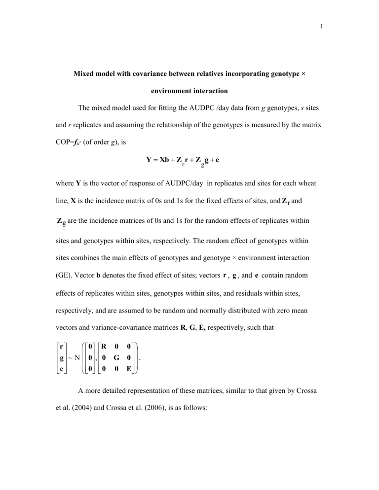
The mixed model used for fitting the AUDPC /day data from g genotypes, s sites and r replicates and assuming the relationship of the genotypes is measured by the matrix
COP= f ii ’
(of order g ), is
Y

Xb

Z r r

Z g g
 e where Y is the vector of response of AUDPC/day in replicates and sites for each wheat line, X is the incidence matrix of 0s and 1s for the fixed effects of sites, and Z r and
Z g are the incidence matrices of 0s and 1s for the random effects of replicates within sites and genotypes within sites, respectively. The random effect of genotypes within sites combines the main effects of genotypes and genotype × environment interaction
(GE). Vector b denotes the fixed effect of sites; vectors r , g , and e contain random effects of replicates within sites, genotypes within sites, and residuals within sites, respectively, and are assumed to be random and normally distributed with zero mean vectors and variance-covariance matrices R , G , E, respectively, such that

 r

 g e




~ N 



0


0
0


,






R
0
0
0
G
0
0
0
E






.
A more detailed representation of these matrices, similar to that given by Crossa et al. (2004) and Crossa et al. (2006), is as follows:
1

2


.


.


.
y
 y


 y
1
2 s













.

.

1 μ


1




.
1
μ
μ
1
2 s






















Z
R
1
0
.
.
.
0
0
Z
R
2
.
.
.
.
.
.
.
.
.
.
.
.
.
.
.
.
.
.
.
.
.
.
.
.
.
0
0
Z
R s










 r












Z
G
1
0
.
.
.
0
0
Z
G
2
.
.
.
.
.
.
.
.
.
.
.
.
.
.
.
.
.
.
.
.
.
.
.
.
.
0
0
Z
G s










 g
 e .
where y is the vector of the response variable in the j j th
site (j=1,2,…, s ); 1 is a vector of ones,
μ is the population mean of the j th
site , j
Z
R j and Z
G j are the design matrices of the random effects of replicates and genotypes within the j th
site, respectively. The variance-covariance matrices R and E are assumed to have the simple variance component structure R
 Σ r

I r
, and E
 Σ e

I rg
where I and r
I are the identity rg matrices of orders r and r
 g , respectively, Σ = r diag( σ
2 r j
, j

1,2,..., s ) and
Σ
= e diag( σ
2 e j
, j

1,2,..., s ) are the s
 s replicate and error variance-covariance matrices among pairs of s sites, respectively; 2 r j
, σ
2 e j are the replicate and residual variances within the j th
site, respectively, and
 is the Kronecker (or direct) product of the two matrices. In covariance pattern models it is assumed that residuals have a multivariate normal distribution with zero means and covariance matrix E.
The variance-covariance matrix G, which combines the main effect of genotypes
(breeding values) and GE, can be represented as:

3
G
 Σ g

A













ρ
12
ρ s
σ
σ
1
σ a
1 a
2 a
.
.
.
s
1
σ
σ a
2 a
1
ρ
12
σ a
1
σ
2 a
2
σ a
2
.
.
.
.
.
.
.
.
.
.
.
.
.
.
.
.
.
.
.
.
.
.
ρ
1 s
σ a
1
σ a s
σ
2
.
.
.
.
a s













A where the j th
diagonal element of the s
 s matrix Σ is the additive genetic g j
within the j th
site, and the ij th
element is the additive genetic covariance
ρ ij
σ a i
σ a j
between sites i and j; thus genetic effects between sites i and j. The matrix A=2 f ii’ is of order g
 g and measures the relationship or covariance between relatives due to additive genetic effects. When genotypes are not related, A is replaced by I (identity matrix of g order g ) (Smith et al., 2002 and Crossa et al., 2004) and the breeding value of each genotype will be predicted only by the value of the empirical response of the genotype itself.
Modeling G and GE of mixed model
The factor analytic structure models covariance among observations in terms of a few hypothetical factors and is useful for modeling matrices G and GE. The unobservable effect of the i th
genotype in the j th
site can be expressed as
1
δ ik x jk
 d ij where
δ is the k th
random regression coefficient of the i th
genotype ik
(loading or genotypic sensitivity) to the k th
unobserved (latent) variable related to the j th

site (environmental potentiality), x , and jk d is the residual interaction term. The score ij
4 of the i th genotype in the k th factor component is estimated as a covariance parameter; thus the model has a random regression coefficient form where x ,
1k x ,…,
2k x s k
are covariates for the k th
factor component. In matrix notation, the vector of genotypic effects is represented by g =
Δ x + d so that the variance-covariance of g is V ( g )=
ΔV
( x )
Δ
'
+ D and, since V ( x )= I, V ( g)= ΔΔ ' + D. The factor analytic model implies that the variance of the effect of the i th
genotype is
 
1
δ
2 ik
 d i and the covariance of the effects of genotypes i and i’ is
1
δ ik
δ i' k
.
The factor-analytic structure with q factors or components [FA( q )] is of the form
ΔΔ
' + D , where
is a s
 q matrix of
δ ’s and
D is a s
 s diagonal matrix with s possibly different non-negative parameters on the diagonal. Each column of
contains the genotype scores for one of the multiplicative terms. For q =1, the model, denoted as
FA(1), has one multiplicative term and 2 s parameters to be estimated, for q =2, i.e., model
FA(2), the model has 3 s parameters to be estimated, and so on for FA(3), etc. In this study we used the FA(2).
Reference Cited
Crossa, J., Burgueño, J., Cornelius, P. L., McLaren, G., Trethowan, R. &
Krishnamachari, A. (2006). Modeling genotype × environment interaction using additive genetic covariances of relatives for predicting breeding values of wheat genotypes. Crop Sci, 46 , 1722-1733.
Crossa, J., Yang, R.-C. & Cornelius, P. L. (2004). Studying crossover genotype× environment interaction using linear-bilinear models and mixed models. J
Agricultural, Biological, and Environmental Statistics, 9 , 362-380.