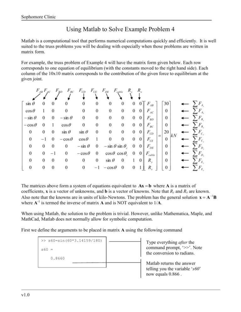
Sophomore Clinic
Using Matlab to Solve Example Problem 4
Matlab is a computational tool that performs numerical computations quickly and efficiently. It is well
suited to the truss problems you will be dealing with especially when those problems are written in
matrix form.
For example, the truss problem of Example 4 will have the matrix form given below. Each row
corresponds to one equation of equilibrium (with the constants moved to the right hand side). Each
column of the 10x10 matrix corresponds to the contribution of the given force to equilibrium at the
given joint.
FAB FAC
 sin 
 cos

  sin 

 cos
 0

 0
 0

 0
 0

 0
FBD
FBC
FCD
FCE
FDE
Fcable
0
1
0
0
0
0
0
0
0
0
0
0
0
0
0
0
 sin 
0
0
0
0
0
1
cos
0
0
0
0
0
0
sin 
sin 
0
0
0
1
0
0
0
 cos
0
cos
 sin 
1
0
0
0
 sin  sin  c
0
1
0
 cos
0
cos cos c
0
0
0
0
0
sin 
0
0
0
0
 1  cos
0
0
Ry
Rx
0 0  FAB  30
0 0  FAC   0 
0 0  FBD   0 
  

0 0  FBC   0 
0 0  FCD  20
    kN

0 0  FCE   0 
0 0  FDE   0 
  

0 0  Fcable   0 
1 0  R y   0 
  

0 1  Rx   0 
F
F
F
F
F
F
F
F
F
F
Ay
Ax
By
Bx
Cy
Cx
Dy
Dx
Ey
Ex
The matrices above form a system of equations equivalent to Ax  b where A is a matrix of
coefficients, x is a vector of unknowns, and b is a vector of knowns. Note that Ry and Rx are known.
Also note that the knowns are in units of kilo-Newtons. The problem has the general solution x  A 1B
where A-1 is termed the inverse of matrix A and is NOT equivalent to 1/A.
When using Matlab, the solution to the problem is trivial. However, unlike Mathematica, Maple, and
MathCad, Matlab does not normally allow for symbolic computation.
First we define the arguments to be placed in matrix A using the following command
>> s60=sin(60*3.14159/180)
s60 =
Type everything after the
command prompt, ‘>>’. Note
the conversion to radians.
0.8660
>>
v1.0
Matlab returns the answer
telling you the variable ‘s60’
now equals 0.866 .
Sophomore Clinic
We should also define ‘c60’ for the cosine of sixty degrees, and‘s30’ and ‘c30’ for the sine and cosine of
thirty degrees. (not shown).
Next we define the matrix A using square brackets ‘[]’. Note the input can be broken arbitrarily across
several lines. The semicolon – ‘;’ – represents the end of a row in the matrix. The comma – ‘,’ –
denotes the next column.
>> A= [s60,0,0,0,0,0,0,0,0,0;c60,1,0,0,0,0,0,0,0,0;-s60,0,0,-s60,0,0,0,0,0,0;
-c60,0,1,c60,0,0,0,0,0,0;0,0,0,s60,s60,0,0,0,0,0;0,-1,0,-c60,c60,1,0,0,0,0;
0,0,0,0,-s60,0,-s60,s30,0,0;0,0,-1,0,-c60,0,c60,c30,0,0;0,0,0,0,0,0,s60,0,1,0;
0,0,0,0,0,-1,-c60,0,0,1]
A =
0.8660
0.5000
-0.8660
-0.5000
0
0
0
0
0
0
0
1.0000
0
0
0
-1.0000
0
0
0
0
0
0
0
1.0000
0
0
0
-1.0000
0
0
0
0
-0.8660
0.5000
0.8660
-0.5000
0
0
0
0
0
0
0
0
0.8660
0.5000
-0.8660
-0.5000
0
0
0
0
0
0
0
1.0000
0
0
0
-1.0000
Before solving the problem we must define the matrix b (see
box at right). The nonzero terms correspond to the external xand y-forces being applied at the corresponding joints.
The final step is to solve the problem with the command
below. We invoke the inverse command, inv, to find
x  A 1B .
The final result is the matrix of unkowns, x, containing our
forces listed by rows in order according to our matrix form
(FAB = 34.6 kN, through Rx = -69.3 kN). They have units
equivalent to b, kilo-Newtons.
>> x=inv(A)*b
x =
34.6410
-17.3205
34.6411
-34.6410
57.7351
-63.5087
-11.5470
80.0001
10.0000
-69.2822
>>
v1.0
0
0
0
0
0
0
-0.8660
0.5000
0.8660
-0.5000
0
0
0
0
0
0
0.5000
0.8660
0
0
0
0
0
0
0
0
0
0
1.0000
0
0
0
0
0
0
0
0
0
0
1.0000
>> b=[30;0;0;0;20;0;0;0;0;0]
b =
30
0
0
0
20
0
0
0
0
0