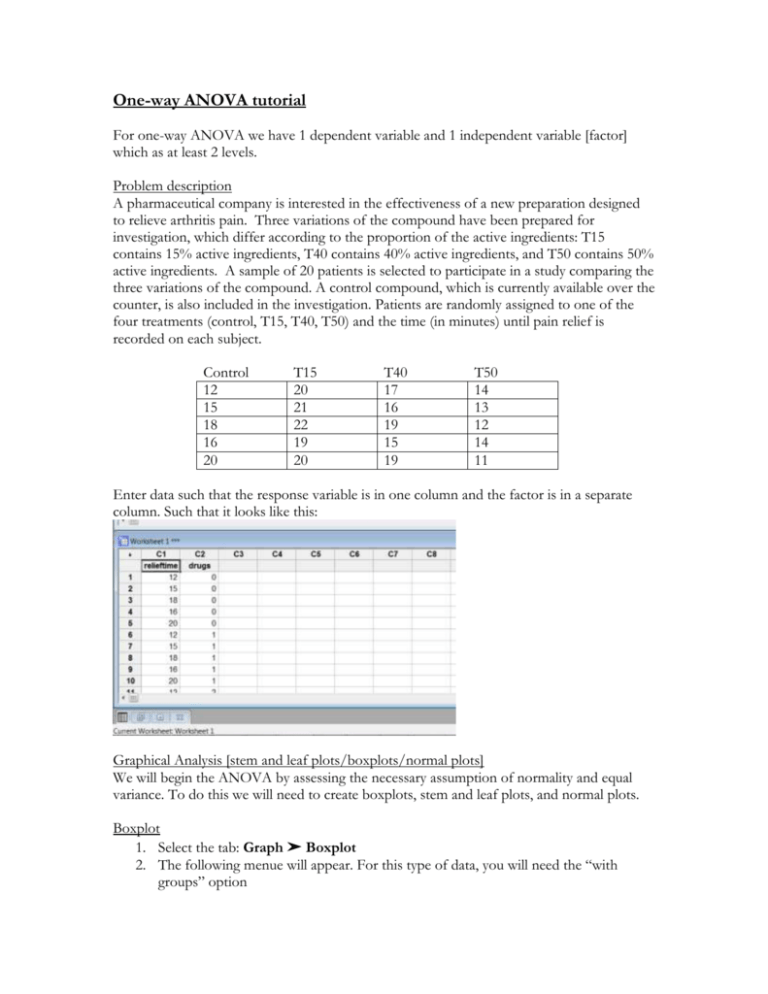
One-way ANOVA tutorial
For one-way ANOVA we have 1 dependent variable and 1 independent variable [factor]
which as at least 2 levels.
Problem description
A pharmaceutical company is interested in the effectiveness of a new preparation designed
to relieve arthritis pain. Three variations of the compound have been prepared for
investigation, which differ according to the proportion of the active ingredients: T15
contains 15% active ingredients, T40 contains 40% active ingredients, and T50 contains 50%
active ingredients. A sample of 20 patients is selected to participate in a study comparing the
three variations of the compound. A control compound, which is currently available over the
counter, is also included in the investigation. Patients are randomly assigned to one of the
four treatments (control, T15, T40, T50) and the time (in minutes) until pain relief is
recorded on each subject.
Control
12
15
18
16
20
T15
20
21
22
19
20
T40
17
16
19
15
19
T50
14
13
12
14
11
Enter data such that the response variable is in one column and the factor is in a separate
column. Such that it looks like this:
Graphical Analysis [stem and leaf plots/boxplots/normal plots]
We will begin the ANOVA by assessing the necessary assumption of normality and equal
variance. To do this we will need to create boxplots, stem and leaf plots, and normal plots.
Boxplot
1. Select the tab: Graph ➤ Boxplot
2. The following menue will appear. For this type of data, you will need the “with
groups” option
3. You then need to select the
appropriate variables. The
graph variable is the dependent
variable. In this example, that
is relieftime. The categorical
variable for grouping is the
independent variable, in this
example: drugs.
4. Select OK
Stem and Leaf
1. Select the Graphs ➤Stem and Leaf
2. The graph variable is again the dependent measure, relieftime. The By variable is the
independent categorical variable, drugs.
3. Select OK
Doing this will give you individual Stem and Leaf plots for each categorical variable. You can
scroll through to see the stem and leaf at drugs = 0, drugs = 1, etc.
To see a Stem and Leaf plot of all dependent data points, simply exclude the “by variable” of
drugs.
You then have the above stem and leaf plot of all data.
Normal probability plot
1. Select Graph ➤Probability plot
2. Your graph variable is relieftime, your
dependent measure
3. Select OK
Note: For separate normal probability plot for each group,
1. Select Graph ➤Probability plot
2. Your graph variable is relieftime, your dependent measure
3. Choose Multiple graphs options ➤choose by variable ➤ move the group
variable to by variable with groups in separate panels
4. Select OK.
Homogeniety of Variance test
1. Select Stat ➤ ANOVA ➤
Test for Equal Variances
2. Again, select variables response variable: relieftime,
factors: drugs
3. Select OK
The test
statistic
appears in the
upper right
hand corner
of the graph
Analysis of Variance - ANOVA
Assuming not problems with our assumptions we can continue by running the one-way
ANOVA.
1. Start by going to Stat ➤ ANOVA ➤
One Way.
2. In Response, enter relieftime. In Factor,
enter drugs.
3. Select OK
Output
Recall that the null hypothesis in ANOVA is that the means of all the groups are the same
and the alternative is that at least one is different . So for our example with 4 treatment
groups
H o : 1   2   3   4
H A : at least one mean is different
To check the hypothesis the computer compares the value for the observed F [12.72] to the
expected value for F-observed given the number of groups and the sample sizes. If this is a
rare event [it will be unusually large is Ho is not true] we will reject Ho. To determine if Fobserved is unusual, we need to look at the (Sig)nificance of the F value [often called the Pvalue]. If this value is less than .05, it means that a score this large would occur less than 5%
of the time [or 1 in every 20 trials] and we will consider it sufficiently rare. The smaller this
value gets the more rare the score and the more certain we can be that the null hypothesis is
incorrect. In the case of above example, we can be confident that if we reject the null
hypothesis, there is less than a 1 in a 1000 chance that we would be incorrect. We limit
ourselves to 1 in a 1000 as [Sig=.000] does not mean that the probability of getting a score
this large is zero, just that its equal to zero at three significant figures
Multiple Comparisons
Post hoc Tests
Using ANOVA table we reject the null hypothesis and conclude that at least one mean is
different from the others. The next question is how they are different. To answer this
question:
1. Start by going to Stat ➤ ANOVA
➤ One Way.
2. Select Comparisons
3. Select the first option, Tukey’s
family error rate
Understanding the
output:
The first set of numbers
provides the overall
results of the test,
organizing in order the
different means of the
groups. The letters
denote statistically
significant differences
between the groups.
The subsequent
sections show the
individual confidence
intervals for each group.
Contrast
A priori contrast: comparisons identified before the experiment has been performed.
For this example we will compare 3 different contrasts
1. Control vs. Compound
2. Low compound (T15) vs. High compound (T40, T50)
3. T40 vs. T50
Creating contrasts: Only requirement is that the sum of the coefficients = 0
1. (1, -1/3, -1/3, -1/3) → (3, -1,-1,-1)
2. (0, 1, -1/2, -1/2) → (0,2,-1,-1)
3. (0,0,1,-1) → (0,0,1,-1)
Step 1 – Link MINITAB to the MACRO library
Step 2 – Enter your contrasts in column format with the coefficient for the first group being
at the top and the coefficients for the last group being at the bottom (there should be as
many coefficients as there are groups – 4 in this case)
1. [3 –1 –1 –1]
2. [0 2 –1 –1]
3. [ 0 0 1 –1]
Step 3 – Run the macro
 Hit “Ctrl+L” to bring up the command line editor
 Type in the macro command with this format
o %contrast C;
o Groups Y X.
 Where C is the column location for the contrast (column 4)
 Where Y is the column location for the response (column 2)
 Where X is the column location for the treatment (column 1)
For this specific example:
Minitab Output (Session Window)
Row
1
2
3
4
Categs
0 5
1 5
2 5
3 5
Freq
16.2
20.4
17.2
12.8
xbar StdDev
3.03315
1.14018
1.78885
1.30384
PooledS 1.96214
alpha
0.950000
---------------CT1
3 -1 -1 -1
Estimated contrast: -1.80000, with standard error 3.03974.
t= -0.59216 (with df= 16); one-sided P-value=0.28101058
Confidence interval: ( -8.24395, 4.64395).
NOTE – We will commonly use a 2-sided P-value so you will need to multiply the 1-sided
P-value by 2 to receive the proper P-value (for this contrast p = 0.562