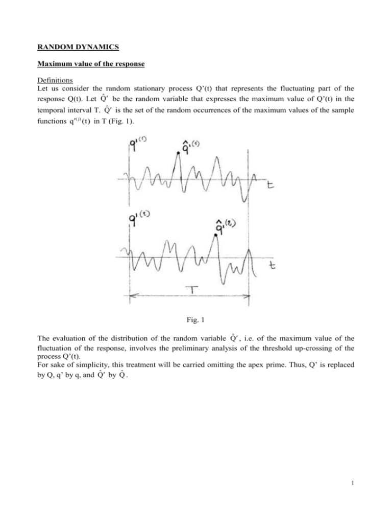
RANDOM DYNAMICS
Maximum value of the response
Definitions
Let us consider the random stationary process Q’(t) that represents the fluctuating part of the
response Q(t). Let Q̂ be the random variable that expresses the maximum value of Q’(t) in the
temporal interval T. Q̂ is the set of the random occurrences of the maximum values of the sample
functions q( j) (t) in T (Fig. 1).
Fig. 1
The evaluation of the distribution of the random variable Q̂ , i.e. of the maximum value of the
fluctuation of the response, involves the preliminary analysis of the threshold up-crossing of the
process Q’(t).
For sake of simplicity, this treatment will be carried omitting the apex prime. Thus, Q’ is replaced
by Q, q’ by q, and Q̂ by Q̂ .
1
Threshold up-crossing of a stationary process
Let us consider a deterministic quantity   0 defined as threshold. Let K   ,T  be the discrete
random variable that counts the number of the up-crossings (+) of the threshold  in the time
interval T (Fig. 2).
Fig. 2
It is demonstrated (Rice 1944, 1945) that the mean value of the up-crossings of the threshold  in
the time interval T is given by:

K  ,T   E K   ,T   T  q pQQ  ,q  dq
0
(1)
where pQQ  q,q  is the joint density function of Q  t  and Q  t  (at the time lag  = 0).
From Eq. (1) it follows that the mean number of the up-crossings up the threshold  in the unit time
is given by:
 N     E  N      
 K   , T 
T

  q p QQ  , q  dq
0
(2)
The solution of Eq. (2) is very simple in the fundamental case in which Q  t  is a normal process.
Let us remember that any stationary process Q  t  and its time derivative Q  t  are uncorrelated for
 = 0, i.e. CQQ (0)  E Q(t)Q(t)   0 . Thus, if Q(t) is a normal process, Q  t  and Q  t  are also
independent (for  = 0). Thus:
2
pQQ  q, q   pQ  q  pQ  q  
2


1
q2 
 q
exp  2  2 
2Q Q

 2Q 2Q 

(3)
Substituting Eq. (3) into Eq. (2), it follows that:
  2 
 N      Q exp  2 
 2Q 
(4)
where:
 Q   N  (0) 
1 Q
2  Q
(5)
is the mean number of the up-crossings of the threshold   0 in the unit time. This quantity is
referred to as the expected frequency of the process.
It is easy to show that the expected frequency Q of a narrow band process is the mean number of
the cycles made by Q(t) in the unit time (Fig. 3).
Fig. 3
Distribution of the maximum (independent threshold up-crossings)
Assuming that the threshold  is high enough, the threshold up-crossings are rare and independent
events (Fig. 4). As such, they are characterised by a Poisson distribution.
Fig. 4
In this case, the probability that the threshold  is up-crossed K+ = n times in the time interval T is
given by:
3
PK   n, , T   exp  K  , T 
  , T 
n
K

n!
(6)
Thus, due to Eq. (2):
T   
  
n!
n
PK   n, , T   exp T N
N

(7)
where, if Q(t) is a normal process,  N    is given by Eq. (4).
Applying Eq. (7) and Eq. (4), the probability that the threshold  is up-crossed K+ = 0 times in the
time interval T is given by:

 2  


PK  0, , T   exp  QT exp   2  
 2Q  



(8)
But the probability that the threshold  is up-crossed K+ = 0 times in the time interval T is equal to
the probability that the maximum value Q̂ of Q  t  in T is less or equal . Thus:
ˆ     P   0, , T 
P Q
K

(9)
ˆ     F    . It follows that the distribution function of the maximum is given by the
being P Q
 Q̂
relationship (Davenport, 1963):

 q̂ 2  
FQˆ  qˆ   exp  Q T exp   2  
 2Q  

(10)
from which, deriving with respect to q̂ , the density function of the maximum value is obtained:
PQˆ  qˆ    Q T

 qˆ 2 
 qˆ 2  
qˆ


exp

exp

T
exp

 2  
 Q
2
2 
Q
 2Q 
 2Q  



(11)
From Eq. (11) it is possible to determine the mean value Q̂ and the standard deviation Q̂ of Q̂ :

Qˆ   qˆ pQˆ  qˆ  dqˆ 
0
Qˆ


0.5772 
Q  2 n   Q T  

2 n  QT  


Q2ˆ  

0
 qˆ   
ˆ
Q
2
(12)
pQˆ  qˆ  dqˆ 
4
Qˆ


Q 
 6



2 n  QT  

1
(13)
Fig. 5 shows the density function of the response process Q(t) and of its maximum Q̂ (on varying
the non-dimensional parameter  Q T ).
Fig. 5
It is worth noting that, on increasing  Q T , the density function of the maximum translates towards
the largest values of q (since Q̂ increases), and its shape becomes more and more narrow and sharp
(since Q̂ diminishes). In other words, on increasing  Q T , Q̂ tends to assume deterministic
properties.
Therefore, when  Q T is small (e.g. in the seismic case), Q̂ is definitely a random variable. When
 Q T is large (e.g. in the wind case), Q̂ may be considered, roughly, as a deterministic quantity
equal to the mean value Q̂ of Q̂ . Using Eq. (12) this value becomes:
Qˆ  gQQ
(14)
where gQ is a non-dimensional quantity referred to as the peak coefficient:
gQ  2 n  QT  
0.5772
2 n  QT 
(15)
Finally, let us remember that all the above analyses refer to the fluctuating part of the response
Q  t  (indicated by Q(t)). Considering also the mean value  Q of the response process, the actual
maximum value is given by (Fig. 6):
5
Qˆ  Q  gQQ
(16)
Fig. 6
Bilateral threshold crossings and absolute maximum value of a normal zero mean process
The above analyses examined the up-crossings the threshold  (Fig. 2). However, in the case of the
normal zero mean processes (e.g. the seismic response), it is relevant to count both the up-crossings
of the threshold  and the down-crossings of the threshold -, i.e. the number of times in which the
process out-crosses the domain (-, ) (Fig. 7). This problem is referred to as the bilateral threshold
crossing.
q
t
Fig. 7
Let N- be the discrete random variable that counts the down-crossings of the threshold - in the unit
time. It is easy to show that  N    N  . Thus, setting N = N+ + N-, then  N   N   N  2 N .
From Eq. (4) it follows that:
6
2
  
 N     2 Q exp  2 
 2Q 
(17)
Based on this new formulation, the distribution function and the density function of the maximum
absolute value Q̂ of Q(t) are given by the relationships:

 q̂ 2  


FQˆ  qˆ   exp 2 QT exp   2  
 2Q  



(18)
2



 qˆ 2  
qˆ
 qˆ 


p Qˆ  qˆ   2 QT 2 exp  2  exp 2 QT exp   2  
Q
 2Q 




 2Q  

(19)
Finally, the mean value and the standard deviation of Q̂ are given by:
 Qˆ  g Q Q
(20)
g Q  2 n  2 Q T  


 Q̂  Q 
 6

0.5772
(21)
2 n  2 Q T 


2 n  2 QT  

1
(22)
Crossings in clumps and envelope process of a narrow band process
Fig. 8 shows a typical sample function of a random stationary normal zero-mean narrow-band
process. It is apparent that the up-crossings of a threshold  tend to occur in clumps. In other words,
any time a sample function up-crosses the threshold, the up-crossing tend to repeat also in the
following cycles.
Fig. 8
In order to understand better this concept, let us consider a new process A(t), the envelope process
of the process Q(t), constituted by the sample functions a(t) (Fig. 9a).
7
Fig. 9
Let NA    be the discrete random variable that counts the up-crossings of the threshold  made by
the process A(t) (Fig. 9b) in the unit time. It is demonstrated that the mean value of NA    results:
q Q Q
  2 
2q Q
 N    
exp  2  
 N   
2
A
Q
2Q
 2Q 
(23)
where q Q is the spectral bandwidth parameter of Q(t).
The mean number of the up-crossings in a clump is referred to as the average clump size. A good
approximation of this quantity is given by the relationship:
cs 
 N   
 N   
A

Q
2q Q
(24)
It is worth noting that cs diminishes on increasing . Thus, on increasing , the threshold upcrossings tend to occur independently.
In the meanwhile, cs is linked with the spectral bandwidth parameter q Q . When the process is
sinusoidal, q Q tends to 0 and cs tends to infinite; in other words, each time the process up-crosses
, the up-crossing repeats infinite other times. On the contrary, when the harmonic content of the
process becomes wider, q Q increases, cs diminishes and the threshold up-crossings tend to
become independent events.
It is worth noting, however, that the limit case in which q Q tends to 1 has no practical meaning in
this context: it is so far from the hypothesis of a narrow band process that all the above treatment
does not apply.
8
Distribution of the maximum (threshold up-crossings in clumps)
The distribution of the maximum value derived above is based on the hypothesis that the threshold
up-crossings are rare and independent events; thus they can be characterised by a Poisson
distribution. Further to this formulation, however, it was noted that this hypothesis is not
appropriate in the case of the narrow band processes, where the threshold up-crossings tend to occur
in clumps. This remark is very important since the dynamic response of the structural systems are
often narrow-band processes. Therefore, it is necessary to generalise the evaluation of the
distribution of the maximum, developed considering independent up-crossings, to the case of upcrossings in clumps.
The most simple way of dealing with this problem is observing that the envelope A(t) up-crosses
the threshold  once per each clump of up-crossings of Q(t) (Fig. 9). So, the threshold up-crossings
of A(t) are really independent events and can be schematised by a Poisson distribution (Lin, 1967).
Paraphrasing the above demonstration (Eq. (7)), the probability that the process A(t) up-crosses the
threshold  K A  n times in the time interval T is given by:
T   
  
n!
n

PN  n, , T   exp T N
A
A
N A
(25)
where  N     is given by Eq. (23). Thus, the probability that A(t) up-crosses the threshold  K A =
A
0 times in the time interval T coincides with the distribution function of the maximum value and is
given by:

 q̂ 2  
2q Q qˆ


FQˆ  qˆ   exp  Q T
exp   2  
Q

 2Q  


(26)
Vanmarcke (1975) perfected this treatment arriving at the following expression of the distribution
function of the maximum value:


  q Q qˆ 
1  exp  



2 Q 
 q̂ 2  


FQˆ  qˆ   exp  Q T
exp   2  
 q̂ 2 
 2Q  

1  exp   2 


 2Q 


(27)
The comparison of Eqs. (10), (26) and (27), considering Eq. (24), points out that Eqs. (26) and (27)
tend to Eq. (10) when cs tends to 1; this is increasingly true on increasing the threshold and the
maximum values considered. Moreover, it is easy to show that Eqs. (26) and (27) tend to Eq. (10)
on increasing  Q T . Under this point of view, Eq. (10) provides better reasonable results in the wind
case, less appropriate solutions in the seismic case.
Finally, it is worth noting that, differently from Eq. (10), Eq. (27) does not allow the derivation of
closed form solutions of the mean value and of the standard deviation of the maximum value. Der
Kiureghian (1980) solved this problem semi-empirically, obtaining the following formulae:
9
Qˆ


0.5772 
Q  2 n   Qe T  

2 n   Qe T  


(28)
 

 

1.2
5.4

per  Qe T  2.1
 Q 
6.4 
Q̂    2 ln   Qe T  13   2 ln  T  
 Qe   

 
0.65
per  Qe T  2.1
Q

(29)
where  Qe is referred to as the reduced expected frequency:
Qe
0.45

1.63q Q  0.38 Q


 Q
per 0.10  q Q  0.69
per q Q  0.69
(30)
Eqs. (28)-(30) apply for 2.5   Q T  500 . Eq. (28) coincides with Eq. (12) for q Q  0.69 . This
confirms that, if the process is broad band, the threshold up-crossings tend to occur independently.
Bilateral threshold up-crossings (in clumps) and absolute maximum values
Generalising Eq. (27), it is easy to show that the distribution of the absolute maximum value Q̂ is
given by the relationship:

  q Q qˆ

1  exp  

 2 Q
FQˆ  qˆ   exp 2 Q T
 q̂ 2 

1  exp   2 

 2Q 





2



q̂
 exp  

2 
 2Q  


(31)
Analogously, generalising Eqs. (28-30), it is easy to show that the mean value and the standard
deviation of Q̂ are furnished by the semi-empirical formulae:
 Q̂


0.5772


Q 2 n  2 Qe T  

2 n  2 QeT  


 

 

1.2
5.4

per 2 Qe T  2.1
 Q 
6.4 
 Q̂    2 ln  2 Qe T  13   2 ln 2 T  
 Qe   

 
0.65
per 2 Qe T  2.1
Q

(32)
(33)
where  Qe is the reduced expected frequency given by Eq. (30).
10