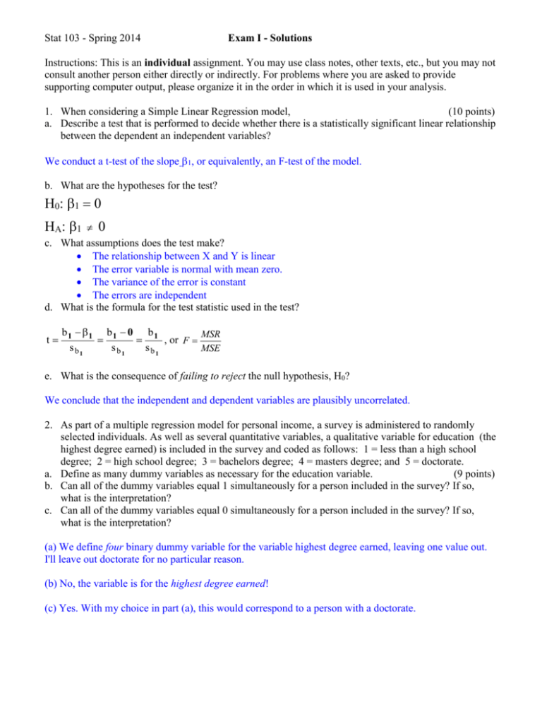
Stat 103 - Spring 2014
Exam I - Solutions
Instructions: This is an individual assignment. You may use class notes, other texts, etc., but you may not
consult another person either directly or indirectly. For problems where you are asked to provide
supporting computer output, please organize it in the order in which it is used in your analysis.
1. When considering a Simple Linear Regression model,
(10 points)
a. Describe a test that is performed to decide whether there is a statistically significant linear relationship
between the dependent an independent variables?
We conduct a t-test of the slope , or equivalently, an F-test of the model
b. What are the hypotheses for the test?
H0: 
HA: 
 0
c. What assumptions does the test make?
 The relationship between X and Y is linear
 The error variable is normal with mean zero.
 The variance of the error is constant
 The errors are independent
d. What is the formula for the test statistic used in the test?
t
b 1  1 b 1  0 b 1
MSR


, or F 
s b1
s b1
s b1
MSE
e. What is the consequence of failing to reject the null hypothesis, H0?
We conclude that the independent and dependent variables are plausibly uncorrelated.
2. As part of a multiple regression model for personal income, a survey is administered to randomly
selected individuals. As well as several quantitative variables, a qualitative variable for education (the
highest degree earned) is included in the survey and coded as follows: 1 = less than a high school
degree; 2 = high school degree; 3 = bachelors degree; 4 = masters degree; and 5 = doctorate.
a. Define as many dummy variables as necessary for the education variable.
(9 points)
b. Can all of the dummy variables equal 1 simultaneously for a person included in the survey? If so,
what is the interpretation?
c. Can all of the dummy variables equal 0 simultaneously for a person included in the survey? If so,
what is the interpretation?
(a) We define four binary dummy variable for the variable highest degree earned, leaving one value out.
I'll leave out doctorate for no particular reason.
(b) No, the variable is for the highest degree earned!
(c) Yes. With my choice in part (a), this would correspond to a person with a doctorate.
3. An agent for a real estate company wishes to use apartment size (in square feet) to predict monthly
rent (in dollars). A sample of 25 apartments in a particular neighborhood led to the following output.
Use the output to answer the questions below.
(2 points each)
Dependent variable: Rent
Independent variable: Size
----------------------------------------------------------------------------Standard
T
Parameter
Estimate
Error
Statistic
P-Value
----------------------------------------------------------------------------Intercept
177.121
161.004
1.1001
0.2827
Slope
1.06514
0.137608
______
0.0000
-----------------------------------------------------------------------------
Analysis of Variance
----------------------------------------------------------------------------Source
Sum of Squares
Df Mean Square
F-Ratio
P-Value
----------------------------------------------------------------------------Model
2.26878E6
1
2.26878E6
59.91
0.0000
Residual
870949.0
23
37867.4
----------------------------------------------------------------------------Total (Corr.)
3.13973E6
24
Correlation Coefficient = 0.850061
R-squared = ________ percent
R-squared (adjusted for d.f.) = 71.0543 percent
Standard Error of Est. = ________
a. What is the equation of the estimated regression line?
Rent = 177 + 1.065*Size
b. What is the t – statistic for the hypothesis test of the slope?
t = b1 / s b1 = 1.06514 / 0.137608 = 7.74
c.
d.
e.
f.
t=
111111111111111111
How many degrees of freedom are associated with the test in part
(b)?
df = n – 2 = 23
111111111111111111
111111111111111111
What is the value of R-squared for the data?
2
R = SSR/SST
= 0.7226
111111111111111111
111111111111111111
What percentage of the variation in the observed rents is explained
by the model?
72.26%
111111111111111111
11fghfghghhfghgf111.
What is the value of S? (include the proper units.)
S = Sqrt(SSE/(n-2))
= $194.60
06514/0.137608
g. Estimate the variance of the error variable for the model
  S2 = (194.6)2 = 37,867
h. Use the regression to estimate the monthly rent of a 1300 square foot apartment in the neighborhood.
Rent = 177.12 + 1.06514*1300 = $1562
i. Interpret the slope of the estimated regression line for this model. Be specific and include units!
Interpretation: For each additional square foot, the rent increases by about $1.065, on average.
j. On the Plot of Residuals vs. Predicted
to the right, circle the observation with
the highest leverage and label it J.
Studentized residual
Residual Plot
k. On the same plot, circle the
observation with the largest absolute
studentized residual and label it K.
3.3
2.3
1.3
0.3
-0.7
-1.7
-2.7
900
1200
1500
1800
2100
2400
predicted Rent
l. Use the graph below to estimate with 95% confidence, to the nearest hundred dollars per month, the
rent of a particular 1300 square foot apartment in the neighborhood. (You may assume that the output
was created using = 0.05.)
Answer: Approx. $1,100 to $2,000
Plot of Fitted Model
2300
Rent
2000
1700
1400
1100
800
700
1000
1300
1600
Size
1900
2200
4. The file HARRIS shows the values of the following variables for 93 employees of Harris Bank
Chicago in 1977:




Salary = beginning (or starting) salary in dollars
Educate = years of schooling at the time of hire
Exper = number of months of previous work experience
Months = number of months after January 1, 1969, that the individual was hired
Construct an initial regression model for the starting salaries of employees of Harris Bank Chicago
using only the variables above. Base all of your responses below on the initial model only!
a. Write down the regression equation for the initial model.
(2 points)
Salary = 3179.74 + 139.618*Educate + 1.4807*Exper + 20.6334*Months
b. Test the overall utility of the model. Explain.
Analysis of Variance
Source
Sum of Squares
Model
1.39844E7
Residual
3.23389E7
Total (Corr.)
4.63233E7
Df
3
89
92
Mean Square
4.66148E6
363358.
F-Ratio
12.83
(4 points)
P-Value
0.0000
The P-value corresponding to the F-Ratio for the model is 0.0000, so the model seems appropriate
pending an analysis of the model assumptions.
c. Are the required conditions satisfied? You do not need to discuss outliers or influential points.(Briefly
summarize your conclusions and provide relevant out for support.)
(4 points)
Variance about the model appears constant, as does the variance about the variables Exper and Months.
Not surprisingly, however, for the variable Educate, there is less variation among those with the least
education. The residuals appear to be nearly normally distributed. Overall, the assumptions are close
enough to being satisfied to proceed.
Residual Plot
Studentized residual
4
2
0
-2
-4
8
10
12
Educate
14
16
Histogram for SRESIDUALS
20
Distribution
Normal
frequency
16
12
8
4
0
-2.5
-0.5
1.5
SRESIDUALS
3.5
5.5
d. Interpret the slopes of each of the independent variables carefully and using the appropriate units.
(6 points)
Salary = 3179.74 + 139.618*Educate + 1.4807*Exper + 20.6334*Months
For each additional year of education, the mean starting salary increases by about $140 per month when
experience and number of months since January 1, 1969 are fixed.
For each additional month of experience, the mean starting salary increases by about $1.50 per month
when education and number of months since January 1, 1969 are fixed.
For each additional months since January 1, 1969, the mean starting salary increases by about $20.60 per
month when education and experience are fixed.
The sex of the employee was also recorded in the dummy variable Male (1 = male). Add the variable
Male to the initial model.
d. Is there evidence, at the 5% level of significance, for a difference in salaries, on average, for male and
female employees at the bank? Explain.
(4 points)
Yes, because the dummy variable Male is significant even after accounting for the employees
education, experience, and date of hire.
e. Interpret the coefficient for the dummy variable Male.
(4 points)
Salary = 3526.42 + 90.0203*Educate + 1.26899*Exper + 23.4062*Months + 722.461*Male
Being male has its advantages! On average, male employees started at $722 per month more than new
female employees having similar education, experience, and hiring date.
f. Predict, with 95% confidence, the mean starting salary for male employees with 12 years of education,
10 years (i.e., 120 months) of experience, and Months = 36 (i.e., hired in December of 1971). Do the
same for females with 12 years of education, 10 years of experience, and Months = 36. Does this
support your conclusion in part (d)? Explain.
(5 points)
Regression Results for Salary
Fitted
Stnd. Error
Row
Value
CL for Forecast
Male
6324.03 527.425
Female 5601.57 520.562
Lower 95.0%
CL for Forecast
5275.88
4567.06
Upper 95.0%
CL for Forecast
7372.18
6636.08
Lower 95.0%
CL for Mean
6038.1
5370.59
Upper 95.0%
CL for Mean
6609.96
5832.54
The intervals for the mean starting salaries for men and women employees of Harris Bank, in dollars,
appear in the table above. Note that the intervals do not overlap! This is clearly supports our previous
conclusion that starting salaries are gender dependent.
5. The editor of an automobile magazine is interested in the effect that a car’s curb weight has on its
highway mileage. The curb weight (in pounds) and highway mileage (in miles per gallon) for 30 cars
is recorded in the file AUTO in the Test 1 folder on your disk.
a. What is the equation of the estimated least squares regression line?
(2 points)
MPG = 46.3298 - 0.00603459*Weight
b. Do curb weight and highway mileage appear to be linearly related? You must justify your answer.
(2 points)
The P-value returned for the model is 0.0000, however, part (c) raises concerns about the appropriateness
of the model.
c. Do the assumptions about the error variable made in the simple linear regression model appear to be
satisfied? You must justify your answer. Include relevant output.
(4 points)
The variance appears to be plausibly constant, and there is no reason to believe the errors are correlated,
but the residuals are skewed to the left, as seen in the graph below, and a test conducted by StatGraphics
rejects the assumption that the errors are normally distributed. Because the sample size isn't particularly
small, some people might not be too concerned with this because the Central Limit Theorem can be
invoked. Still, for such a strongly skewed distribution we might want to be cautious.
Density Trace for SRESIDUALS
0.4
density
0.3
0.2
0.1
0
-3
-2
-1
0
1
2
SRESIDUALS
Histogram for SRESIDUALS
8
Distribution
Normal
frequency
6
4
2
0
-3.2
-2.2
-1.2
-0.2
SRESIDUALS
0.8
1.8
Tests for Normality for SRESIDUALS
Test
Statistic
P-Value
Shapiro-Wilk W
0.911952
0.0182557
The StatAdvisor
This pane shows the results of several tests run to determine whether SRESIDUALS can be adequately modeled by a normal distribution.
The Shapiro-Wilk test is based upon comparing the quantiles of the fitted normal distribution to the quantiles of the data.
Since the smallest P-value amongst the tests performed is less than 0.05, we can reject the idea that SRESIDUALS comes from a normal
distribution with 95% confidence.