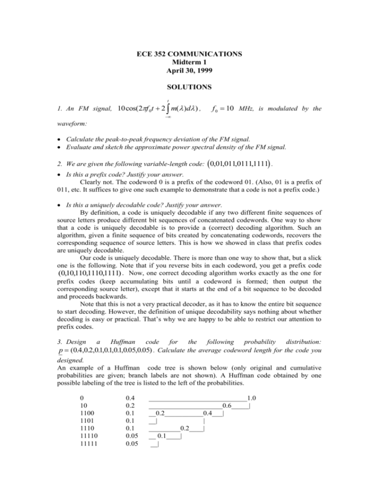
ECE 352 COMMUNICATIONS
Midterm 1
April 30, 1999
SOLUTIONS
t

1. An FM signal, 10 cos(2f 0t  2 m( )d ) ,
f 0  10 MHz, is modulated by the

waveform:
 Calculate the peak-to-peak frequency deviation of the FM signal.
 Evaluate and sketch the approximate power spectral density of the FM signal.
2. We are given the following variable-length code: 0,01,011,01111111
,
.
 Is this a prefix code? Justify your answer.
Clearly not. The codeword 0 is a prefix of the codeword 01. (Also, 01 is a prefix of
011, etc. It suffices to give one such example to demonstrate that a code is not a prefix code.)
 Is this a uniquely decodable code? Justify your answer.
By definition, a code is uniquely decodable if any two different finite sequences of
source letters produce different bit sequences of concatenated codewords. One way to show
that a code is uniquely decodable is to provide a (correct) decoding algorithm. Such an
algorithm, given a finite sequence of bits created by concatenating codewords, recovers the
corresponding sequence of source letters. This is how we showed in class that prefix codes
are uniquely decodable.
Our code is uniquely decodable. There is more than one way to show that, but a slick
one is the following. Note that if you reverse bits in each codeword, you get a prefix code
(0,10,110,1110,1111) . Now, one correct decoding algorithm works exactly as the one for
prefix codes (keep accumulating bits until a codeword is formed; then output the
corresponding source letter), except that it starts at the end of a bit sequence to be decoded
and proceeds backwards.
Note that this is not a very practical decoder, as it has to know the entire bit sequence
to start decoding. However, the definition of unique decodability says nothing about whether
decoding is easy or practical. That’s why we are happy to be able to restrict our attention to
prefix codes.
3. Design
a
Huffman
code for the following probability distribution:
p  (0.4,0.2,01
. ,01
. ,01
. ,0.05,0.05) . Calculate the average codeword length for the code you
designed.
An example of a Huffman code tree is shown below (only original and cumulative
probabilities are given; branch labels are not shown). A Huffman code obtained by one
possible labeling of the tree is listed to the left of the probabilities.
0
10
1100
1101
1110
11110
11111
0.4
0.2
0.1
0.1
0.1
0.05
0.05
____________________________1.0
_____________________0.6_____|
__0.2___________0.4___|
__|
|
_________0.2____|
__ 0.1____|
__|
l  0.4  1  0.2  2  01
.  4  01
.  4  01
.  4  5  0.05  5  0.05  2.5 bits per source letter.
4. Given a source with the two letter alphabet A  a, b , parse the following string into
phrases using LZ78. Also, show a tree built as a result of the parsing. The string:
aaabbabbababababbba.
In LZ78, the part of the string that has not been parsed yet is processed as follows.
We go down the tree, matching source letters from the string with branch labels, as long as
we can. Then we output the number of a node we reached that way and the first unmatched
source letter. The tree is then expanded by adding to the node a new branch ending with a
new node. The new branch is labeled with the source letter and the new node is assigned the
next available number. Initially, the tree has no branches and just one node whose number is
0.
5. Draw the partition for the nearest neighbor vector quantizer whose codebook is
(0,0),(1,0),(2,0),(1,0),(2,0),(0,1),(0,2), (0,1),(0,2) .
In the nearest neighbor quantizer each sample (vector) to be quantized is assigned to
the closest representation value (ties can be resolved arbitrarily).
6. Draw a block diagram of the DPCM encoder and decoder.
7. Which of the following statements are true?
 DPCM can take advantage of sample-to-sample correlation. TRUE. Correlation is exactly
what DPCM is supposed to take advantage of.
 The average codeword length of a Huffman code must be an integer. FALSE. See solution
to problem 3.
 The typical way the real numbers are represented in computers is an example of uniform
quantization. FALSE. Roughly speaking, the length of a quantization bin is proportional to
the magnitude of the numbers contained in the bin, and so is not constant.
 The Lloyd algorithm is based on the nearest neighbor condition and the centroid
condition. TRUE. In the Lloyd iteration we calculate a new codebook based on the centroid
condition and then calculate a new partition based on the nearest neighbor condition.
 Every uniquely decodable code is a prefix code. FALSE. See solution to problem 2.
8. Prove that if each probability pi from a source probability distribution vector can be
expressed as pi  2
 ki
for some integer ki , then the average codeword length for a Huffman
code for this source is equal to its entropy: l  H ( p) .
J 1
J 1
0
0
 2 ki   pi  1. Hence, the vector of integers (k0 , k1 ,, k J 1 )
We have
satisfies Kraft’s inequality. Therefore, there exists a prefix code (c0 , c1, , cJ 1 ) such that
k
the length of the codeword ci is ki . Now, note that ki   log2 2 i  log 2 (1 / pi ) . The
average codeword length is l 
J 1
J 1
0
0
 pi ki  pi log2 (1/ pi )  H( p) . Since the average
codeword length of a Huffman code is not greater than that of (c0 , c1, , cJ 1 ) and not less
than H ( p) , our conclusion follows.
9. Let X and Y be two random variables with probability distributions p and q ,
respectively. The quantity called mutual information
I ( X ; Y )    pi , j log
i
j
pi , j
pi q j
I ( X ; Y ) is defined as
pi , j  P( X  ai , Y  bj ) are probabilities from
, where
the joint probability distribution of X and Y .
 What is I ( X ; Y ) if X and Y are independent. If X and Y are independent,
pi , j  pi q j . Since log(1)  0 , we have that I ( X ; Y )  0 in that case. We can interpret that
by saying that if X and Y are independent, then by observing Y we don’t get any
information about X (and vice versa; note that I ( X ; Y )  I (Y; X ) ).
 What is I ( X ; X ) . I ( X ; X )  H( X ) . One can easily prove it. However, the easiest way
to find out what I ( X ; X ) is during the exam would be to look at the equality below when
Y  X . Using the interpretations we developed in class, H( X , X )  H( X ) (observing X
“twice” gives us as much information as observing it “once”). The conclusion follows
immediately.
 Prove that H( X ; Y )  H( X )  H(Y )  I ( X ; Y ) . From probability theory we have
pi   pi , j and q j   pi , j .
i
j
H( X )  H(Y )  I ( X ; Y ) 
 p log(1 / p )  q
i
i
i
 p
i, j
i
j
j
j
log(1 / q j )    pi , j log(
log(1 / pi )    pi , j log(1 / q j )    pi , j log(
j
i
i
j
i
pi , j
pi q j
)
j
pi , j
pi q j
)
 p
i, j
i
j
log(
1 1 pi q j
)  H( X ; Y ) .
pi q j pi , j