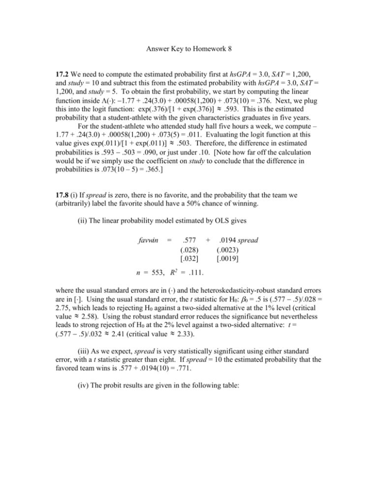
Answer Key to Homework 8
17.2 We need to compute the estimated probability first at hsGPA = 3.0, SAT = 1,200,
and study = 10 and subtract this from the estimated probability with hsGPA = 3.0, SAT =
1,200, and study = 5. To obtain the first probability, we start by computing the linear
function inside (): 1.77 + .24(3.0) + .00058(1,200) + .073(10) = .376. Next, we plug
this into the logit function: exp(.376)/[1 + exp(.376)]  .593. This is the estimated
probability that a student-athlete with the given characteristics graduates in five years.
For the student-athlete who attended study hall five hours a week, we compute –
1.77 + .24(3.0) + .00058(1,200) + .073(5) = .011. Evaluating the logit function at this
value gives exp(.011)/[1 + exp(.011)]  .503. Therefore, the difference in estimated
probabilities is .593  .503 = .090, or just under .10. [Note how far off the calculation
would be if we simply use the coefficient on study to conclude that the difference in
probabilities is .073(10 – 5) = .365.]
17.8 (i) If spread is zero, there is no favorite, and the probability that the team we
(arbitrarily) label the favorite should have a 50% chance of winning.
(ii) The linear probability model estimated by OLS gives
favwin
=
.577
(.028)
[.032]
+
.0194 spread
(.0023)
[.0019]
n = 553, R2 = .111.
where the usual standard errors are in () and the heteroskedasticity-robust standard errors
are in []. Using the usual standard error, the t statistic for H0: 0 = .5 is (.577  .5)/.028 =
2.75, which leads to rejecting H0 against a two-sided alternative at the 1% level (critical
value  2.58). Using the robust standard error reduces the significance but nevertheless
leads to strong rejection of H0 at the 2% level against a two-sided alternative: t =
(.577  .5)/.032  2.41 (critical value  2.33).
(iii) As we expect, spread is very statistically significant using either standard
error, with a t statistic greater than eight. If spread = 10 the estimated probability that the
favored team wins is .577 + .0194(10) = .771.
(iv) The probit results are given in the following table:
Dependent Variable: favwin
Independent
Variable
spread
Coefficient
(Standard Error)
.0925
(.0122)
.0106
(.1037)
constant
Number of Observations
Log Likelihood Value
Pseudo R-Squared
553
263.56
.129
In the Probit model
P(favwin = 1|spread) = (0 + 1spread),
where () denotes the standard normal cdf, if 0 = 0 then
P(favwin = 1|spread) = (1spread)
and, in particular, P(favwin = 1|spread = 0) = (0) = .5. This is the analog of testing
whether the intercept is .5 in the LPM. From the table, the t statistic for testing H0: 0 = 0
is only about -.102, so we do not reject H0.
(v) When spread = 10 the predicted response probability from the estimated
probit model is [-.0106 + .0925(10)] = (.9144)  .820. This is somewhat above the
estimate for the LPM.
(vi) When favhome, fav25, and und25 are added to the probit model, the value of
the log-likelihood becomes –262.64. Therefore, the likelihood ratio statistic is
2[262.64 – (263.56)] = 2(263.56 – 262.64) = 1.84. The p-value from the  32
distribution is about .61, so favhome, fav25, and und25 are jointly very insignificant.
Once spread is controlled for, these other factors have no additional power for predicting
the outcome.