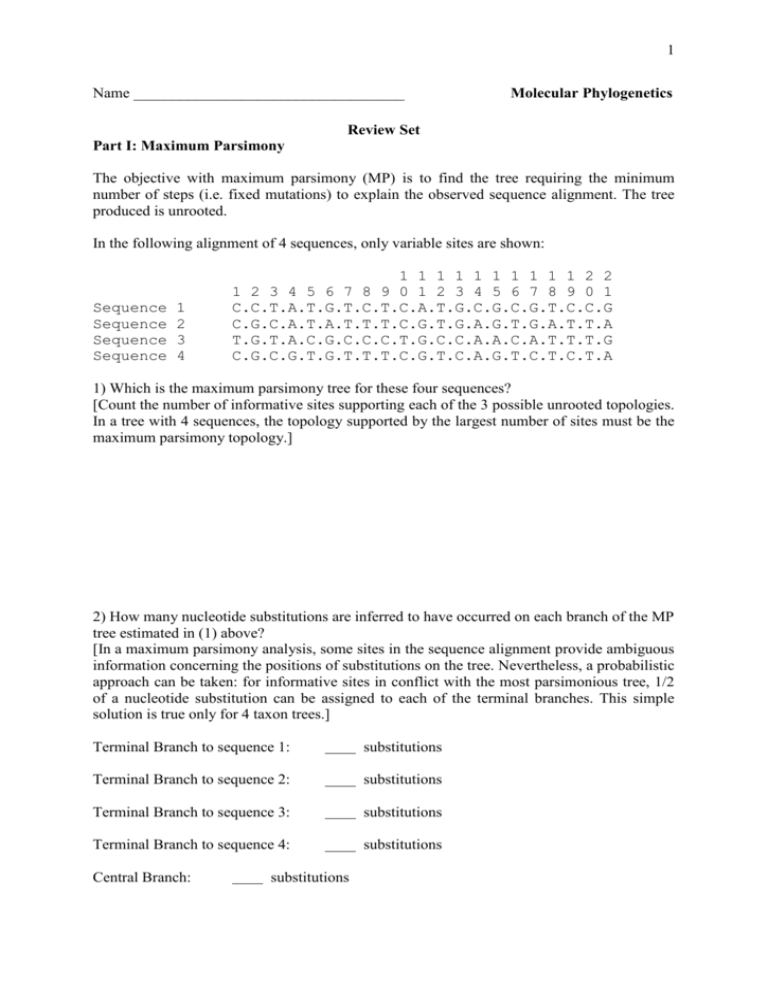
1
Name ___________________________________
Molecular Phylogenetics
Review Set
Part I: Maximum Parsimony
The objective with maximum parsimony (MP) is to find the tree requiring the minimum
number of steps (i.e. fixed mutations) to explain the observed sequence alignment. The tree
produced is unrooted.
In the following alignment of 4 sequences, only variable sites are shown:
Sequence
Sequence
Sequence
Sequence
1
2
3
4
1 1 1 1 1 1 1 1 1 1 2 2
1 2 3 4 5 6 7 8 9 0 1 2 3 4 5 6 7 8 9 0 1
C.C.T.A.T.G.T.C.T.C.A.T.G.C.G.C.G.T.C.C.G
C.G.C.A.T.A.T.T.T.C.G.T.G.A.G.T.G.A.T.T.A
T.G.T.A.C.G.C.C.C.T.G.C.C.A.A.C.A.T.T.T.G
C.G.C.G.T.G.T.T.T.C.G.T.C.A.G.T.C.T.C.T.A
1) Which is the maximum parsimony tree for these four sequences?
[Count the number of informative sites supporting each of the 3 possible unrooted topologies.
In a tree with 4 sequences, the topology supported by the largest number of sites must be the
maximum parsimony topology.]
2) How many nucleotide substitutions are inferred to have occurred on each branch of the MP
tree estimated in (1) above?
[In a maximum parsimony analysis, some sites in the sequence alignment provide ambiguous
information concerning the positions of substitutions on the tree. Nevertheless, a probabilistic
approach can be taken: for informative sites in conflict with the most parsimonious tree, 1/2
of a nucleotide substitution can be assigned to each of the terminal branches. This simple
solution is true only for 4 taxon trees.]
Terminal Branch to sequence 1:
substitutions
Terminal Branch to sequence 2:
substitutions
Terminal Branch to sequence 3:
substitutions
Terminal Branch to sequence 4:
substitutions
Central Branch:
substitutions
2
3) When alternative types of nucleotide substitution do not occur at equal frequencies, it may
be better to perform “weighted maximum parsimony”. For example in mammalian
mitochondrial DNA, transitions are thought to occur (at least) 10 times as often as
transversions. Therefore, to weight we could count each transversional change as worth 10
transitions. If we do this, which is the maximum parsimony tree?
3
Part II: Distances and UPGMA Trees
The objective of this exercise is to calculate distances and build a UPGMA tree for the
following group of sequences:
1
Seq1
Seq2
Seq3
Seq4
Seq5
Seq6
50
GATTGCCTTG
..........
AG........
...C......
...G......
..CC......
GATCCTTGAC
..........
..........
A.C.......
A.C.......
..G.....G.
TGATCGGGTC
.....A....
.....A....
.A....A...
.A....A...
......AC..
GCTTGCTACC
..........
..........
..........
..........
...C...G..
TTACAGCGAT
..........
.G..G...G.
.G..T.....
.G..C..A..
.C..G..C..
1) Count the number of differences
Seq1
Seq2
Seq3
Seq4
Seq5
Seq6
Seq1
-
Seq2
Seq3
Seq4
Seq5
Seq6
-
2) Calculate the uncorrected p distances
Seq1
Seq2
Seq3
Seq4
Seq5
Seq6
Seq1
-
Seq2
Seq3
Seq4
Seq5
Seq6
-
3) Correct the distances to account for multiple hits using the Jukes Cantor (JC) model.
Kxy = - 3/4 ln (1 – 4/3 d)
Where:
Kxy = estimated number of nucleotide substitutions per site between sequence x and
sequence y [estimated distance between sequence x and sequence y]
d = observed proportion of nucleotides that differ between the 2 sequences
Seq1
Seq2
Seq3
Seq4
Seq5
Seq6
Seq1
-
Seq2
Seq3
Seq4
Seq5
Seq6
-
4
4) The distances below were estimated using the F84 model. This model is very similar to the
HKY85 model and allows transitions and transversions to have different rates as well as
allowing for unequal base frequencies.
Seq1
Seq2
Seq3
Seq4
Seq5
Seq6
Seq1
Seq2
Seq3
Seq4
Seq5
0.0202
0.1311
0.1558
0.1824
0.2643
0.1075
0.1798
0.2073
0.2914
0.2286
0.2578
0.3589
0.0622
0.2705
0.3043
Seq6
How do the distances estimated using the F84 model differ from those estimated using the JC
model?
Which model do you think is more appropriate for the sequence data and why?
5) Draw the UPGMA tree for the 6 sequences based on the distance matrix in #4.
5
6) The neighbour-joining tree for these 6 sequences is given below:
How do the UPGMA and NJ trees differ?
7) Based on observations of the sequence data and your knowledge of the assumptions of
UPGMA and NJ, which tree do you think is most accurate and why?
8) It is known that sequences 1 and 2 diverged 2 million years ago. Calculate the rate of
substitution using the distances in (3).
r = K/2T
where:
r = rate of substitution (number of substitutions per site per year)
K = number of substitutions between 2 sequences
T = time since divergence of the 2 sequences
6
9) Assuming a molecular clock, calculate the age of :
a) the divergence of sequences 1+2 from 3
b) the divergence of sequences 1+2 from 4+5 (excluding 3)
10) In a relative rates test, we can compare the rates in two closely related species (or clades
of species), A and B, with a third more distantly related outgroup species (or clade of
species), C, as a reference.
KAC = average distance between A and the outgroup taxon C
KBC = average distance between B and the outgroup taxon C
If KAC-KBC = 0 then both lineages are evolving at the same rate. Anything other than 0, then
one lineage is evolving faster than the other.
Conduct a relative rates test to determine whether:
a) sequence 3 is evolving at the same rate as sequences 1 and 2
b) sequences 4 and 5 are evolving at the same rate as sequences 1 and 2
11) Is it appropriate to use a molecular clock to estimate the time of
a) the divergence of sequences 1+2 from 3?
b) the divergence of sequences 1+2 from 4+5 (excluding 3)?
7
Part III. Bacterial Phylogenies
a) Comparing Tree Topologies
Eight evolutionary trees are shown overleaf. The same eight species of bacteria appear in
each, but each tree was derived from analysis of a different protein.
Species
Gene
Length Protein
Escherichia coli
Haemophilus influenzae
Neisseria meningitidis
Pasteurella multocida
Pseudomonas aeruginosa
Vibrio cholerae
Xylella fastidiosa
Yersinia pestis
rpoA
recA
rpsA
ffh
mopA
rplB
tpiA
tufA
327
343
545
450
541
271
243
394
DNA- directed RNA polymerase alpha subunit
RecA recombination protein
30S ribosomal subunit protein S1
signal recognition particle protein
chaperonin 60kD subunit (GroEL)
50S ribosomal subunit protein L2
triosephosphate isomerase
elongation factor Tu
Neisseria meningitidis is placed in the beta proteobacteria; the other seven species are
classified as gamma proteobacteria. The length given is the number of aligned amino acid
sequences.
Tree methods used: after multiple sequence alignment, a matrix of pairwise distances was
constructed; distances were corrected for multiple hits by Kimura’s empirical method. The
trees were then estimated by Neighbour-joining (NJ) analysis. NJ defines the tree topology
and branch lengths but produces an unrooted tree.
1) In the rpoA tree, which species is/are the most closely related to Vibrio cholerae?
2) The majority of the eight trees have identical topologies. Which trees have different
topologies, and how do they differ from the consensus topology?
3) What are the possible reasons for differences in topology among these trees?
4) How might you root the tree? Which of the trees looks like the best representation of a
rooted tree for these species?
8
rpoA
recA
mopA
rplB
rpsA
tpiA
ffh
tufA
9
b) Neighbour Joining Analysis with Bootstraps
The sequence of the infC gene encoding translation initiation factor 3 is available for
15 different species of gamma proteobacteria. These predicted protein sequences
together with that from Neisseria meningitidis were analysed by the NJ method as on
the previous pages. The infC gene is very unusual in that analysis of the E. coli gene
has revealed that its translation initiation codon is ATT. In other bacterial species,
other unusual codons are used: the inferred translation initiation codons for each
species are given here:
1. Buchnera sp. APS
2. Buchnera aphidicola
3. Escherichia coli
4. Haemophilus influenzae
5. Klebsiella pneumoniae
6. Neisseria meningitidis
7. Pasteurella multocida
8. Proteus vulgaris
ATT
ATT
ATT
ATT
ATT
ATC
ATT
ATT
9. Pseudomonas aeruginosa
10. Pseudomonas fluorescens
11. Pseudomonas syringae
12. Salmonella typhimurium
13. Serratia marcescens
14. Vibrio cholerae
15. Xylella fastidiosa
16. Yersinia pestis
ATC
ATT
ATT
ATT
ATT
ATT
ATC
ATT
Neisseria meningitidis is placed in the beta proteobacteria; the other fifteen species
are classified as gamma proteobacteria.
The results of the NJ analysis are summarised below. The NJ method progresses
through n-2 rounds (where n is the number of sequences), inserting a new internal
branch in each round until a fully bifurcating tree is produced. Each time a new
branch is inserted it implies that 2 sequences (or 2 clades of sequences) have been
joined at one end of the branch.
The notation below is output from the NJ tree construction program NEIGHBOR of
the PHYLIP package. It indicates which sequences (or clades) are joined in each
round, and shows the branch length from that node to the sequence (or clade). In this
notation, clades are referred to as ‘nodes’ on the tree and are given a number referring
to the lowest numbered sequence within that clade.
round
round
round
round
round
round
round
round
round
round
round
round
round
round
1 :
2 :
3 :
4 :
5 :
6 :
7 :
8 :
9 :
10:
11:
12:
13:
14:
seq 10 (0.008) joins seq 11 (0.010)
seq 9 (0.063) joins node 10 (0.054)
seq 6 (0.197) joins seq 15 (0.361)
seq 4 (0.025) joins seq 7 (0.030)
node 6 (0.092) joins node 9 (0.181)
seq 1 (0.050) joins seq 2 (0.058)
node 4 (0.132) joins node 6 (0.056)
node 4 (0.024) joins seq 14 (0.160)
seq 13 (0.035) joins seq 16 (0.021)
seq 3 (0.003) joins seq 12 (0.003)
node 3 (0.006) joins seq 5 (0.018)
seq 8 (0.074) joins node 13 (0.035)
node 1 (0.063) joins node 3 (0.037)
node 1 (0.006) + node 4 (0.054) + node 8 (0.009)
10
For example, in round 1, sequence 10 (see above) joins sequence 11 at the first node.
The branch length from this node to sequence 10 is 0.008 and to sequence 11 is 0.010.
In round 2, sequence 9 joins node 10 (i.e., the clade formed by sequences 10 and 11)
at a second node. The branch length from this second node to sequence 9 is 0.063 and
from the second node to the first node is 0.054.
The output can also be represented in the form of a treefile:
((((((10:0.008,11:0.010):0.054,9:0.063):0.181,(6:0.0197,15:0.361):0.092):0.056,(4:0.0
25,7:0.030):0.132):0.024,14:0.160):0.054,((1:0.050,2:0.058):0.063,((3:0.003,12:0.003
):0.006,5:0.018):0.037):0.06,((13:0.035,16:0.021):0.035,8:0.074):0.009);
1) Draw out the full tree
[Do this roughly at first, concentrating on the topology only. Then draw out a neater
version with branch lengths roughly to scale. Remember that the tree is unrooted!
11
2) Re-draw the tree as a rooted tree by rooting on an appropriate outgroup taxon.
3) An alternative approach to rooting a tree is to assume an approximate molecular
clock, and then root at the midpoint of the longest pairwise distance implied by the
tree. In this tree, the longest pairwise distance is from Buchnera aphidicola to Cylella
fastidiosa. The distance is given by the sum of all the branches connecting these
species (0.058 + 0.063 + 0.006 + 0.054 + 0.024 + 0.056 + 0.092 + 0.361 = 0.714).
With midpoint rooting, on which branch of the tree does the root lie? How does this
compare with the outgroup rooting above?
12
4) One thousand bootstrap replicates were examined to assess the support for the infC
tree. The matrix below shows the results. Each column refers to a sequence. Each row
refers to a partition in the tree (i.e., a branch separating 2 clades) between the
sequences indicated by * in one clade and the sequences indicated by – in the other
clade. The value at the right on each row is the number of bootstrap replicates in
which the partition was found.
1234
****
****
****
*******
--**
**********
**-*
**-*
****
---*
5678
****
****
*-**
**-*
*-**
****
*--*
*--*
****
****
-***
***-***
111
9012
*--*
---*
****
****
---*
****
---*
---*
****
**********
***-
1111
3456
****
****
**-*
****
**-*
****
**-*
*--*
-******
****
-******
1000
1000
945
999
845
1000
654
991
979
709
998
443
393
Place the bootstrap values on the tree in (2)
5) Is the tree topology obtained for infC consistent with any of those found on page 8?
If yes, which? If no, how does it differ?
6) What is the minimum number of times that the nature of the translation initiation
codon must have changed on the infC NJ tree?
7) Do the three Pseudomonas species form a monophyletic group in the infC NJ tree?
If so, can this clade be considered to be well-supported or poorly supported in the
analyses of the infC dataset?
8) Do Vibrio, Haemophilus and Pasteurella form a monophyletic group in the infC NJ
tree? If so, can this clade be considered to be well-supported or poorly-supported in
analyses of the infC dataset?
9) Is the grouping of Escherichia/Salmonella/Klebsiella with the Buchnera species in
the infC NJ tree reliable?