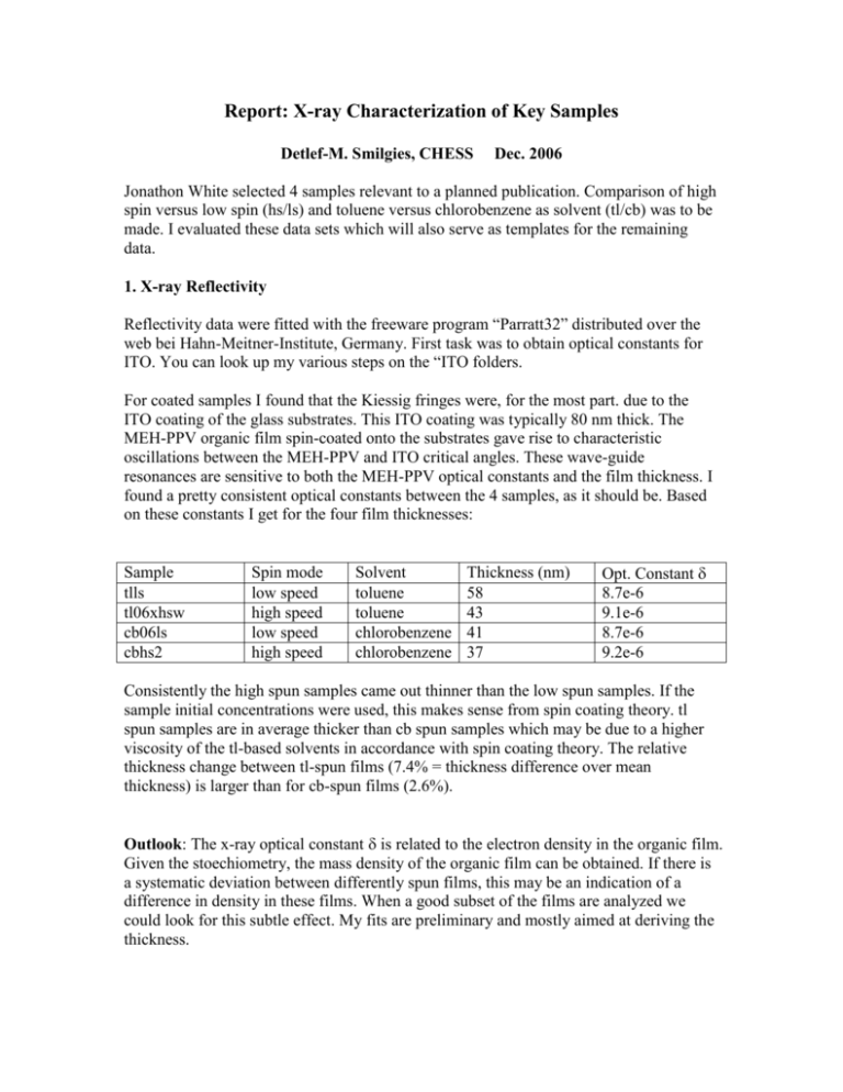
Report: X-ray Characterization of Key Samples
Detlef-M. Smilgies, CHESS
Dec. 2006
Jonathon White selected 4 samples relevant to a planned publication. Comparison of high
spin versus low spin (hs/ls) and toluene versus chlorobenzene as solvent (tl/cb) was to be
made. I evaluated these data sets which will also serve as templates for the remaining
data.
1. X-ray Reflectivity
Reflectivity data were fitted with the freeware program “Parratt32” distributed over the
web bei Hahn-Meitner-Institute, Germany. First task was to obtain optical constants for
ITO. You can look up my various steps on the “ITO folders.
For coated samples I found that the Kiessig fringes were, for the most part. due to the
ITO coating of the glass substrates. This ITO coating was typically 80 nm thick. The
MEH-PPV organic film spin-coated onto the substrates gave rise to characteristic
oscillations between the MEH-PPV and ITO critical angles. These wave-guide
resonances are sensitive to both the MEH-PPV optical constants and the film thickness. I
found a pretty consistent optical constants between the 4 samples, as it should be. Based
on these constants I get for the four film thicknesses:
Sample
tlls
tl06xhsw
cb06ls
cbhs2
Spin mode
low speed
high speed
low speed
high speed
Solvent
toluene
toluene
chlorobenzene
chlorobenzene
Thickness (nm)
58
43
41
37
Opt. Constant 
8.7e-6
9.1e-6
8.7e-6
9.2e-6
Consistently the high spun samples came out thinner than the low spun samples. If the
sample initial concentrations were used, this makes sense from spin coating theory. tl
spun samples are in average thicker than cb spun samples which may be due to a higher
viscosity of the tl-based solvents in accordance with spin coating theory. The relative
thickness change between tl-spun films (7.4% = thickness difference over mean
thickness) is larger than for cb-spun films (2.6%).
Outlook: The x-ray optical constant  is related to the electron density in the organic film.
Given the stoechiometry, the mass density of the organic film can be obtained. If there is
a systematic deviation between differently spun films, this may be an indication of a
difference in density in these films. When a good subset of the films are analyzed we
could look for this subtle effect. My fits are preliminary and mostly aimed at deriving the
thickness.
2. GIWAXS
I recalibrated thr GIWAXS camera, and obtained the following new parameters:
- wavelength: 1.19156 A
- detector distance: 101.5 mm
- beam center: has to be determined for each GIWAXS image series – usually the direct
beam image is the last one in a series.
My calibration procedures are shown in the “behenate” folder.
GIWAXS images of the four samples feature a reflection at 15.2 nm-1 corresponding to a
d-spacing of 0.41 nm, typically ascribed to the -stacking of the aromatic polymer
backbone. Scans of the radial wavevector integrated of an azimuthal range of 90 deg
(perpendicular to the sample) to 180 deg (parallel to the sample) reveal a sharper peak on
a broad background. Using more selective integration ranges, maybe the broad and sharp
components could be studied in more detail.
Scans of the azimuth obtained by integrating images over a large radial range (300 to 900
pixels from the direct beam) reveal a relatively broad distribution with a half-width-athalf-maximum (HWHM) of 40 to 45 deg. This means that the Bragg planes have a only a
weak tendency to aligned parallel to the substrate surface.
Some structure in the azimuth distributions seems to appear also in the parallel direction,
however, need further analysis. The sharp peak close to 180 deg, i.e. grazing exit angle, is
the so-called Yoneda peak when the x-rays are scattered at an exit angle corresponding to
the film critical angle. This peak is of dynamic nature (i.e. related to the scattering
process) and not relevant to the discussion of preferential orientations.
Further analysis using the fit2d CAKE feature (see my fit2d primer on the web) could be
done varying azimuthal and radial integration ranges.
A summary of the integrated scans is given on the main folder “key-samples” for the
comparison of radial and azimuth intensity distributions (files “GIWAXS-radial-widths”
and “GIWAXS-azimuth-widths”).
Outlook: For this analysis I selected images from each sample with an exposure of 10
sec and an incident angle set to the first minimum past the organic film critical angle.
This meant I had to choose different images in two cases than Jonathon originally
selected by carefully tracing back all information contained in the logfiles. There is an
extra 10-20% variation due to the decay of the positron beam in the storage ring which I
have not yet accounted for, but also is contained in the log file (“CESR” and “Imon”
columns). Nonetheless it is quite evident, both in the 2D images and the integrated scans,
that the two tl-spun samples scatter very differently. Part of this could be due to poor
alignment of the hs sample which is harder to retrace. When we get to evaluating the
other samples, we should investigate whether this behavior of the tl-hs film is systematic
or a fluke.
3. Transformation of 2D images to reciprocal space
At present fit2D does not have a built-in feature that transforms WAXS data into
reciprocal space. I include a sample file how this task can be achieved with Origin, which,
however, is infinitely slower than fit2D. For publication purposes, the image can be
binned 5x5 (or even 10x10), i.e. 5x5 pixels are averaged to yield a new pixel. Even then
Origin transforms are slow compared to the 2D CAKE transformation by fit2d. Hence
use of the Origin-based transforms should only by made for publication-style figures. For
easier viewing of images, I made a mirror image of the original image, to move the data
from the 2nd quadrant to the first. So far I have only treated sample “tlls”. The Origin
spreadsheet has comments on the various steps and Origin features used (requires Origin
7.0 or higher. Origin 6 regridding routines are slow and unstable.)
In the case of SAXS data the transform can be linearized, and we only have to rescaled
the axes from pixels to inverse nm. This can be done using the “MATRIX > set
dimension” feature in Origin or axis rescaling in fit2d which I have to relearn. I include
two calculations “q-transform-WAXS” and “q-transform SAXS” that illustrate this.
4. GISAXS data
I have not yet had a chance to look into these images. I have devoted almost 4 days of
analysis in getting points 1. to 3. taken care of. Now I have to tend to some other urgent
things. Let me know when you are ready to look at SAXS data, and I will find some time
to get you started.