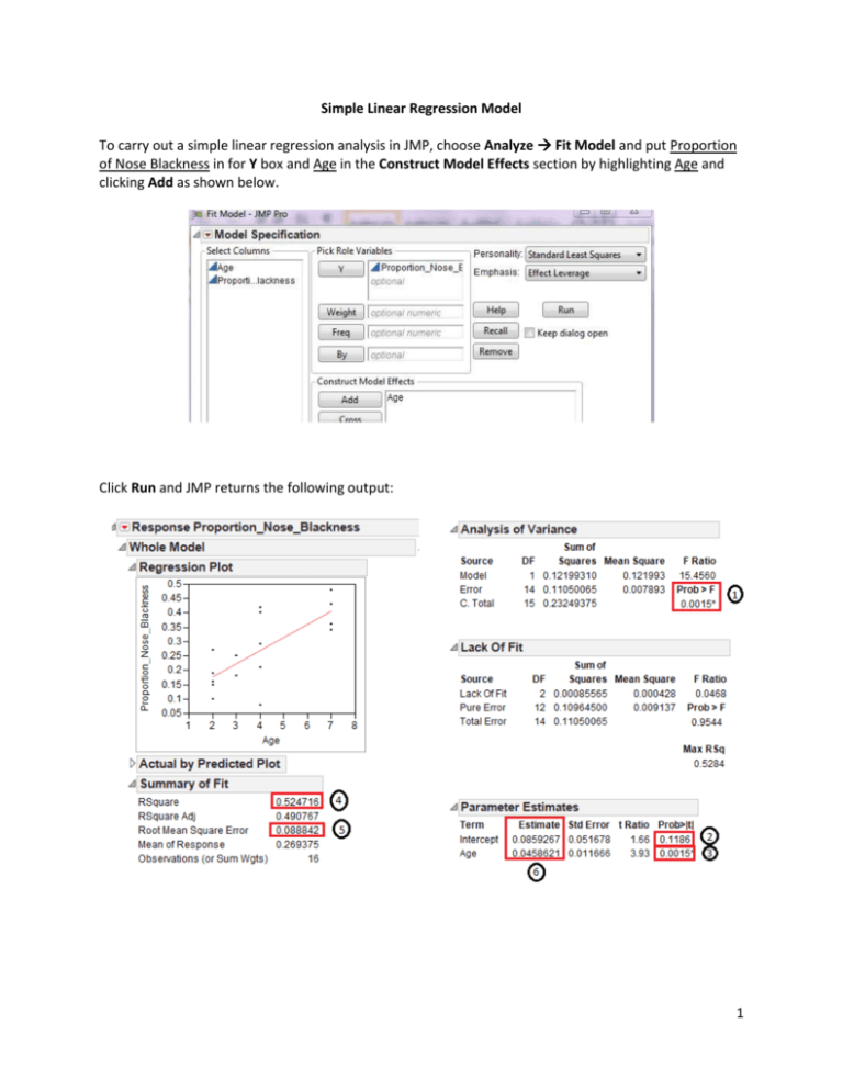
Simple Linear Regression Model
To carry out a simple linear regression analysis in JMP, choose Analyze  Fit Model and put Proportion
of Nose Blackness in for Y box and Age in the Construct Model Effects section by highlighting Age and
clicking Add as shown below.
Click Run and JMP returns the following output:
1
Understanding the JMP regression output:
This p-value tests whether or not the overall regression is useful.
H0: Regression model is _____ useful
Ha: Regression model _____ useful
p-value -
Conclusion -
These p-values test hypotheses concerning both the intercept and slope.
and
Intercept
H0: Intercept = 0
Ha: Intercept ≠ 0
Slope
H0: slope = 0
Ha: slope ≠ 0
p-value –
p-value –
conclusion –
conclusion –
2
This is the called the coefficient of determination usually called R-Square (R2).
This quantity measures the percent of total variation in the y-variable that can
be explained by the x-variable.
R2 =
Interpretation –
This is the Root Mean Square Error (RMSE). This quantity estimates the
average distance of a data point from the fitted line, measured along the
vertical axis. Such a distance is known as a residual.
The smaller the RMSE, the better the fit of the model.
RMSE =
These values give the estimates of both the intercept and the slope so that we
can write the equation of the fitted line.
Ê (Proportion of Nose Blackness | Age) = 0.086 + 0.046*Age
3
Interpretations of these values
Slope:
Intercept:
Predicting the Mean of Y | X
To use the lion’s age to predict the proportion of nose blackness, we simply use the equation:
Ê (Proportion of Nose Blackness | Age) = 0.086 + 0.046*Age
For example, to predict the proportion of nose blackness for a 4 year-old lion:
Next, predict the proportion of nose blackness for a 5 year-old lion.
4
To get the predicted values (and the residuals) from JMP, choose Save Columns  Predicted Values and
Save Columns  Residuals from the red drop-down arrow.
Assumptions behind a simple linear regression analysis
The assumptions behind the analysis are as follows:
1. The response variable (y) and the predictor variable (x) have a ______________________
relationship. That is, y can be modeled using x in the following form:
E(Y | X) = β0 + β1 x
2. The variability in the response (y) must be the same for each x.
Good
Bad
5
3. The response measurements (y) should be _____________________ of each other.
4. The response measurements (y) should be _____________________ distributed.
5. You should also take the time to identify outliers. These can be very problematic in a regression
analysis.
Fitted Line WITH Outlier
Fitted Line WITHOUT Outlier
How to check the regression assumptions
We can check the first three assumptions listed below by creating t a scatterplot with the residuals on
the y-axis and the predicted values on the y-axis.
Ideal Residual Plot:
Violations to Assumption #1 (Linearity):
Some existing trend remaining (BAD)
Some nonlinear trend remaining (BAD)
6
Violations to Assumption #2 (Constant Variance):
Fan Shape opening to right (BAD)
Fan Shape opening to the left (BAD)
Violations to Assumption #3 (Independence):
One point closely following another –
positive autocorrelation (BAD)
Extreme bouncing back and forth –
negative autocorrelation (BAD)
Violations to Assumption #4 (Normality):
To check this, click on the red drop-down arrow and select Save Residuals. Then, make a histogram
of the residuals and/or look at a normal quantile plot. Recall that you can easily make a histogram
or a normal quantile plot of a variable in JMP using the Analyze  Distribution menu.
Checking for outliers:
Determine the value of 2*RMSE. Then, look at the residual plot once more and draw a horizontal
reference line at both ± 2*RMSE. Any observations outside these bands are potential outliers and
should be investigated further to determine whether or not they adversely affect the model.
7
Checking the assumptions for the lion data
As we’ve seen previously, JMP automatically provides a plot of the residuals versus the predicted values.
Check the following assumptions based on this plot of the residuals versus the predicted values.

Linearity:

Constant variance:

Independence:
8
Next, we can look at a histogram of the residuals of the normal quantile plot to assess for normality.
What can you say about the assumption of normality?
Finally, does there appear to be any potential outliers?
9