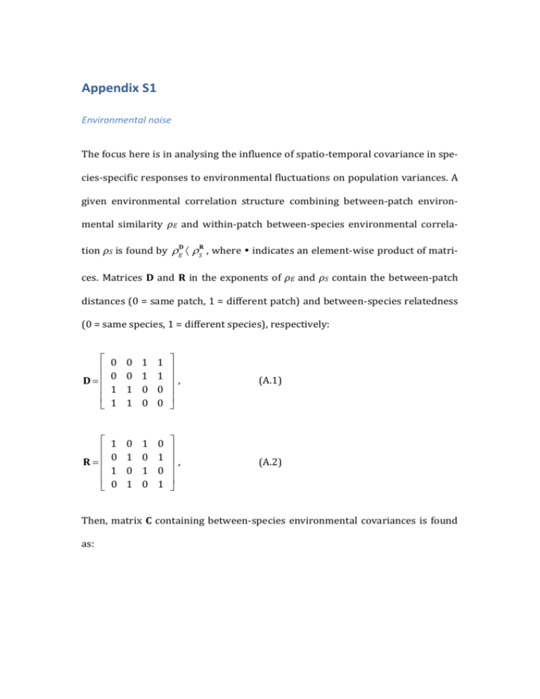
Appendix S1
Environmental noise
The focus here is in analysing the influence of spatio-temporal covariance in species-specific responses to environmental fluctuations on population variances. A
given environmental correlation structure combining between-patch environmental similarity ρE and within-patch between-species environmental correlaD
R
tion ρS is found by rE · r S , where  indicates an element-wise product of matri-
ces. Matrices D and R in the exponents of ρE and ρS contain the between-patch
distances (0 = same patch, 1 = different patch) and between-species relatedness
(0 = same species, 1 = different species), respectively:
é
ê
D= ê
ê
ê
ë
0
0
1
1
0
0
1
1
1
1
0
0
1
1
0
0
ù
ú
ú,
ú
ú
û
(A.1)
é
ê
R=ê
ê
ê
ë
1
0
1
0
0
1
0
1
1
0
1
0
0
1
0
1
ù
ú
ú,
ú
ú
û
(A.2)
Then, matrix C containing between-species environmental covariances is found
as:
é 1
ê
ê rE
C = s 2 rED · r SR = s 2 ê
ê rS
ê
êë rE rS
rE r S ù
rE
rS
1
rE r S
rS
rE r S
1
rE
rS
rE
1
ú
ú
ú,
ú
ú
úû
(A.3)
where σ2 is the environmental variance. The exponentiation of ρE and ρS with D
an R, respectively, is made element-wise. As a result, zeros in matrices D and R
become replaced with ones, whereas the ones are replaced by ρE and ρS, respectively. The resulting covariance matrix C is positive definite for all combinations
of ρE and ρS (which is required for the covariance structure to be feasible), as
long as |ρE, ρS | < 1. The combined term ρEρS describing the environmental correlation between species between patches, which dependence on ρE and ρS is illustrated in Figure S1.
Population variance
For analytically deriving within-patch population variances, several matrices
controlling different ecological processes, need to be defines. For describing between-patch dispersal, a dispersal matrix is needed:
(1 − 𝑚11 )
0
𝑚12
0
0
(1 − 𝑚21 )
0
𝑚22
𝐌=[
] ,
𝑚11
0
(1 − 𝑚12 )
0
0
𝑚21
0
(1 − 𝑚22 )
(A.4)
This dispersal matrix can be combined with the Jacobian matrix, describing local
dynamics, to form a metacommunity matrix:
𝐁 = 𝐌𝐉 ,
where J is the Jacobian matrix of the local communities:
(A.5)
𝐉=[
𝐉1
𝟎
𝟎
].
𝐉2
(A.6)
Here Ji is the jacobian for local community i and 0 is a matrix of zeros of the
same size as Ji (here 2 x 2 in size).
Assuming that patches are identical (population parameters are independent of spatial location), species equilibrium densities become independent
of the movement parameter mik. This simplification makes it possible to find the
metacommunity matrices for each system. The local Jacobian matrices Ji are defined as follows.
Competition model:
𝜃𝑟
𝐉𝑖 = [
𝛼𝜃𝑟
1 − 𝛼+1
− 𝛼+1
],
𝜃𝑟
1 − 𝛼+1
𝛼𝜃𝑟
− 𝛼+1
(A.7)
consumer–resource model:
1+
𝑑𝑟(𝑒𝑎(𝑅0 −𝐾)+𝑅0 𝑑+𝐾𝑑)
𝐾𝑎𝑒(𝑑−𝑎𝑒)
𝑑𝑟(𝑅0 +𝐾)
𝐉𝑖 = [
𝑒𝑟 −
−𝑑𝑒
],
(A.8)
1
𝐾𝑎
host–parasitoid model:
𝐉𝑖 = [
𝑞𝑟(𝑟 −1/𝑞 −1)
1
1
1−𝑟
−
𝑟−1
]
𝑞(𝑟 −1/𝑞 −1)
.
(A.9)
𝑟−1
In the absence of environmental autocorrelation (κ = 0) population variances can be found analytically by first transforming system dynamics to run
along the eigenvectors of B (Ripa and Ives, 2003). For this a matrix T, with each
column representing an eigenvectors of B, as well as the eigenvalues λi of B. The
variance-covariance matrix in the eigenvector space Υ is then found as (Ripa and
Ives, 2003):
𝛾
𝜈𝑖𝑗 = 1−𝜆𝑖𝑗𝜆 ,
(A.10)
𝑖 𝑗
where γij indicate the elements of the transformed environmental covariance
matrix C: Γ = T–1C(T–1)T. Population variances can be obtained by a backtransformation from eigenvector space to population coordinates, V = TΥT–1,
where V is the population variance-covariance matrix. Using this method population variance in the competitive metacommunity becomes:
𝑉=
𝜎2 (𝜌𝐸 +1)(𝜌𝑆 −1)
2[
𝜆21 −1
Θ
−
(𝜌𝐸 +1)(𝜌𝑆 +1)
𝜆22 −1
−
(𝜌𝐸 −1)(𝜌𝑆 −1)
𝜆23 −1
+
(𝜌𝐸 −1)(𝜌𝑆 +1)
𝜆24 −1
],
(A.11)
where σ is the SD of environmental noise. Under symmetric dispersal (mik = m)
the Jacobian eigenvalues are: λ1 = (α – θr + αθr + 1)/(α + 1), λ2 = 1 – θr, λ3 = [α(θr
+ 1) – 2m(θr – αθr – α – 1) – θr + 1]/ (α + 1), λ4 = 2m(θr – 1) – θr + 1. Parameter
Θ is the order of matrix B (here Θ = 4). Eqn. (A.11) is actually just the sum of the
variances along the Jacobian eigenvectors divided by the number of eigenvectors, i.e., a mean over the variances in eigenvector space.
Ideally, it should be possible to partition population variance into components depending on ρE and ρS alone, and their interaction ρEρS. In the absence
of the interaction term the independent components are easily obtained, by setting α = 0 or m = 0, respectively:
𝜎2 𝜌𝐸 −1
𝑉|𝛼=0 =
Θ
𝑉|𝑚=0 =
𝜌 +1
(A.12a)
( 𝜆2 −1 − 𝜆𝐸2 −1 )
1
2
𝜎2 𝜌𝑆 −1
(
Θ 𝜆24 −1
𝜌 +1
− 𝜆2𝑆−1) .
(A.12b)
2
Eqn. (A.11) can be rearranged to display the interrelation between the
Jacobian eigenvalues, and ρE, ρS and ρEρS, including a term that is independent of
the environmental correlation structure:
𝑉=
𝜎 2 𝜌𝐸
Θ
2
1
3
𝜎 2 𝜌𝐸 𝜌𝑆
+
1
1
1
(𝜆2 −1 + 𝜆2 −1 − 𝜆2 −1 − 𝜆2 −1) +
2
Θ
4
1
1
2
1
1
1
𝜎 2 𝜌𝑆
Θ
2
(𝜆2 −1 + 𝜆2 −1 − 𝜆2 −1 − 𝜆2 −1) −
1
4
2
3
1
1
1
1
(𝜆2 −1 + 𝜆2 −1 − 𝜆2 −1 − 𝜆2 −1)
1
𝜎2
Θ
2
3
∑4𝑖=1
1
𝜆2𝑖 −1
2
4
.
(A.13)
Here it becomes more clear that the effect of ρE depends on the relative strength
of dispersal mediated processes (λ3 and λ4) and local processes (λ1 and λ2),
whereas the effect of ρS depends on the relative strength of interspecific interaction (λ1 and λ3) and intrinsic density regulation (λ2 and λ4). Finally, how the magnitude of the interaction term ρEρS depends on different processes is not that
clear. The magnitude of the eigenvalue-sum that multiplies the ρEρS term increase with increasing θ and r, decreases with α, and decreases (increases) with
m when intrinsic dynamics are undercompensatory (overcompensatory).
An analytical expression for population variance in autocorrelated environments is also possible to derive (Ripa and Ives, 2003; Ruokolainen and Ripa,
2012):
𝑉=
𝜎2 (𝜆2 𝜅+1)(𝜌𝐸 +1)(𝜌𝑆 +1)
Θ
2
[
−
(𝜆22 −1)(𝜆2 𝜅−1)
−
(𝜆3 𝜅+1)(𝜌𝐸 −1)(𝜌𝑆 −1)
(𝜆23 −1)(𝜆3 𝜅−1)
(𝜆1 𝜅+1)(𝜌𝐸 +1)(𝜌𝑆 −1)
(𝜆21 −1)(𝜆1 𝜅−1)
+
(𝜆4 𝜅+1)(𝜌𝐸 −1)(𝜌𝑆 +1)
(𝜆24 −1)(𝜆4 𝜅−1)
],
(A.14)
where κ is the environmental autocorrelation. Systems with potentially complex
eigenvalues and eigenvectors, such as eqns. A.8 and A.9, are harder to solve (Ripa
and Ives, 2003). The solutions (if even obtainable) are very complex (due to the
Jacobian eigenvectors being dependent on model parameters), so they will not
be treated here.
Supplementary References
Ripa, J., Ives, A.R., 2003. Food web dynamics in correlated and autocorrelated environments. Theor. Popul. Biol. 64, 369–384.
Ruokolainen, L., Ripa, J., 2012. The strength of species interactions modifies population responses to environmental variation in competitive communities. J. Theor. Biol. 310, 199–205.