Linear Algebra and TI 89
Abdul Hassen and Jay Schiffman
This short manual is a quick guide to the use of TI89 for Linear Algebra. We do this in two sections. In
the first section, we will go over the editing of matrices and vectors. The second section will address the
algebraic operations of Linear Algebra. To make the manual short and useful, we have assumed that the reader
is familiar with the keyboard and the functions of the SECOND, ALPHA, DIAMOND GREEN keys as well
as the use of CATALOG. The reader should also be familiar with the usages of the “cursor” keys to move form
one option to another in a given menu. Note also that some menus have several submenus, which in turn may
have many options.
1.
EDITING MATRICES AND VECTORS
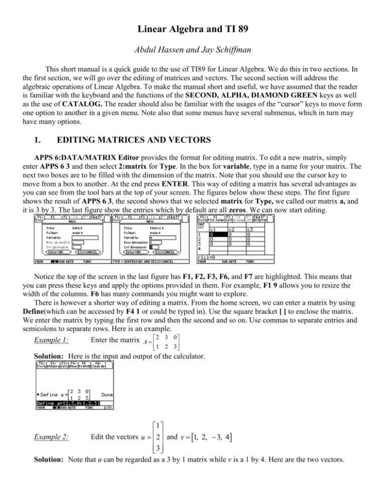
APPS 6:DATA/MATRIX Editor provides the format for editing matrix. To edit a new matrix, simply
enter APPS 6 3 and then select 2:matrix for Type. In the box for variable, type in a name for your matrix. The
next two boxes are to be filled with the dimension of the matrix. Note that you should use the cursor key to
move from a box to another. At the end press ENTER. This way of editing a matrix has several advantages as
you can see from the tool bars at the top of your screen. The figures below show these steps. The first figure
shows the result of APPS 6 3, the second shows that we selected matrix for Type, we called our matrix a, and
it is 3 by 3. The last figure show the entries which by default are all zeros. We can now start editing.
Notice the top of the screen in the last figure has F1, F2, F3, F6, and F7 are highlighted. This means that
you can press these keys and apply the options provided in them. For example, F1 9 allows you to resize the
width of the columns. F6 has many commands you might want to explore.
There is however a shorter way of editing a matrix. From the home screen, we can enter a matrix by using
Define(which can be accessed by F4 1 or could be typed in). Use the square bracket [ ] to enclose the matrix.
We enter the matrix by typing the first row and then the second and so on. Use commas to separate entries and
semicolons to separate rows. Here is an example.
Example 1:
Enter the matrix A   2 3 0
1 2 3
Solution: Here is the input and output of the calculator.
1 
Example 2:
Edit the vectors u   2  and v  1, 2,  3, 4
 
 3 
Solution: Note that u can be regarded as a 3 by 1 matrix while v is a 1 by 4. Here are the two vectors.
2.
OPERATIONS ON MATRICES
We begin with examples of matrix operations.
Example 3:
 1 2
A

 1 0 
Consider the following matrices.
 1 2 3
9 1 
B
C   0 2 1 

0 3
 2 0 3 
1 3 1 
1 1 0
1 0 6 

D
E   2 3 4
7 0 1 
1 0 2


2 2 1 
If possible, compute each of the following.
A B
a)
b)
3 A - 4B
DE
ED
e)
f)
T
i)
j)
A B
Solution:
1
2 
3 
1 2
1 3
F 
1 3

0 1
c)
g)
A B
E C
3 2
0 2 
2 0

4 3
d)
h)
AC
D E  F2
1 2 3
 1 2 3
1 3 0
 1 2



Example 4:
Find the inverse of the matrices A  
 , B   0 2 1  and C  1 3 0

1
0


 2 0 3 

0 1 4
Solution: Enter the matrices and then from the HOME screen evaluate A ^ ( 1) , B ^ ( 1) and C ^ (1) .
Note that for C ^ (1) the output is error: Singular matrix.
Example 5:
of B.
2
2 
2

3
Let B be as in Example 4. Find the 2-3 entry, the diagonal entries, first row, and second column
Solution:
Enter the matrix as b. For the j-k entry use b[j,k], for first row use b[1], and for the
T
second column use b [2] , where the T in the exponent is for the transpose of b.
Example 6(Special Matrices)
(a) Generate a 2 by 3 random matrix.
b) Generate a 3 by 3 identity
matrix.
Solution.
a) Use MATH 4 E to display randMat( and then type 2,3) and evaluate. For b) either type or
use MATH 4 6 to display identity( and then type 3 and evaluate.
3
SOLVING SYSTEMS OF LINEAR EQUATIONS
Example 7
Solve the system of linear equations.
 x yz 3
x  3y  2z  1

a)
b)
c)

 2x  3 y  4z  1
 x  2y  z  4
3x  6 y  5 z  2

Soution:
From the home screen press MATH 4 5. This gives simult(. Next we enter the
coefficients and the constant matrix as below.( Recall that we enter a matrix by typing the first row and then the
second and so on. Use commas to separate entries and semicolons to separate rows.)
x  y 1

x  y  3
Note that for c) we got an error message as we notice above. We might want to try the elementary row
operations to solve this problem. To do this, we define the coefficient matrix as A and the constant matrix as B
and then apply rref(augment(A,B)). The rref command can be accessed by Math 4 4 while augment can be
obtained by MATH 4 7.
We leave it to the reader to interpret this output.
4.
Vector Operations
1 
1 


Example 8:Let u  2 and v  3  . Find u  v , u  v , ||v|| and the unit vector in the direction of u.
 
 
 3 
9 
Solution:
Enter the vectors as in Example 2 above. Then MATH 4 L 3 will display dotP(. Now
type u,v) and ENTER. The result is the dot product; in this case it is 34. Similarly MATH 4 L 2 u,v) ENTER
will give the cross product. For the norm of v use MATH 4 H 1 v) ENTER. Finally, to find the unit vector in
the direction of u,we use MATH 4 L 1 u) ENTER. The first figure below shows the result of defining the
vectors, the second shows the dot and the cross products and the last one shows the norm of v and the unit
vector in the direction of u.
5.
Eigenvalues and Eigenvectors
Example 9
Find the eigenvalues and eigenvectors for the following matrices
1 2 3 2 
 1 2 3
1 3 0 2 
 2 1
0 2 1


 2 3
D

B

C

 2 0
A





1

3
2
0


1 2 


 2 0 3 
0 1 4 3 
Solution:
We use the define option to enter the matrices as a, b, c, and d, respectively. To find the
eigenvalues of the matrix A, use Math 4 9 a ) ENTER or type eigvl(a) and ENTER. To find the eigenvectors
of the matrix a use Math 4 A a ) ENTER or type eigvc(a). The figure below shows the eigenvalues and
eigenvectors of the matrix A.
Remark:
1.
2.
The first number given by eigVl(a) is the first eigenvalue which in this case is -1 and second
eigenvalue is 1. The first column of the eigVc(a) is an eigenvector corresponding to the first
eigenvalue of a. Note that TI 89 is normalizing the vectors, that is the eigenvectors are unit
vectors.
For most purposes and easier notations, it is convenient to rewrite the eigenvectors with integer
entries. This is usually possible. One possible method is to replace the smallest number in the
columns by 1 and divide the other entries in that column by the smallest value you just replaced.
Use the command eigVc(a)[j,k] to refer to the j-k entry of the matrix eigVc(a). It is clear that the
entries in the first column are equal. Thus for an eigenvector corresponding to the eigenvalue -1,
we may take 1 . The second one may not be clear so we replace -.316228 by 1. Note then that 1
.96683/-.316228 is 3.062. Thus it is highly recommended that you compute eigVc(a)[2,1]/
eigVc(a)[2,2]. We find that this is 3. Thus we may take 3 as the second eigenvector.
1
 
If we evaluating eigvl(b), we will get the message Non-real result. This means that the characteristic equation
of the matrix B has complex roots. Note that we could use the command cSolve(det( b – x*identity(2))=0,x)
ENTER, we get the complex eigenvalues, namely, x  1  i or x  1  i as shown below.
6.
Applications
Example 10.
Let v1 , v2 , v3 , v4 be the vertices of the complete graph on four vertices. Find the
determinant and eigenvalues of the graph.
Solution: Note that the determinant and eigenvalues of a graph are the determinant and eigenvalues of the
adjacency matrix. The adjacency matrix is defined as the matrix A   aij  , where

1, if vi , v j  is an edge of the graph
aij  

0, otherwise
0 1 1 1 
1 0 1 1 
 . We enter this
For the complete graph on four vertices, the adjacency matrix is given by A  
1 1 0 1 


1 1 1 0 
matrix as a and evaluate det(a) to get 3 as the determinant of the graph and evaluate eigvl(a) to get
{3, 1, 1, 1} as the eigenvalues of the graph.
Example 11: Find the number of walks of length 3 from v1 to v3 .
Solution:
Again we use the adjacency matrix as defined in example 10 above. The number of walks of
length 3 from v1 to v3 is given by the (1,3) entry of the cube of the adjacency matrix A. As in example 10, we
6 7 7 7 
7 6 7 7 
3
3
 . Thus the (1,3) entry is
enter the adjacency matrix as a and evaluate a to obtain the matrix A  
7 7 6 7 


7 7 7 6 
7. Hence there are 7 walks of length 3 from v1 to v3 in the complete graph on four vertices. We leave it to the
reader to list the seven walks.