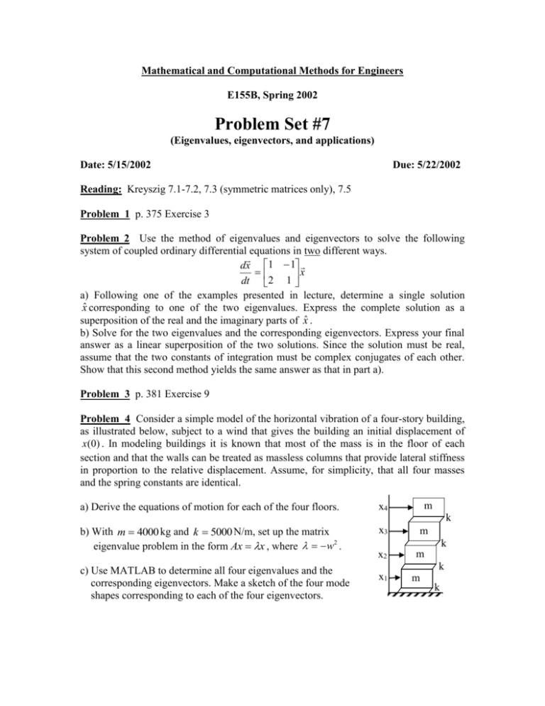
Mathematical and Computational Methods for Engineers
E155B, Spring 2002
Problem Set #7
(Eigenvalues, eigenvectors, and applications)
Date: 5/15/2002
Due: 5/22/2002
Reading: Kreyszig 7.1-7.2, 7.3 (symmetric matrices only), 7.5
Problem 1 p. 375 Exercise 3
Problem 2 Use the method of eigenvalues and eigenvectors to solve the following
system of coupled ordinary differential equations in two different ways.

dx 1  1 

x
dt 2 1 
a) Following one of the examples presented in lecture, determine a single solution
x̂ corresponding to one of the two eigenvalues. Express the complete solution as a
superposition of the real and the imaginary parts of x̂ .
b) Solve for the two eigenvalues and the corresponding eigenvectors. Express your final
answer as a linear superposition of the two solutions. Since the solution must be real,
assume that the two constants of integration must be complex conjugates of each other.
Show that this second method yields the same answer as that in part a).
Problem 3 p. 381 Exercise 9
Problem 4 Consider a simple model of the horizontal vibration of a four-story building,
as illustrated below, subject to a wind that gives the building an initial displacement of
x (0) . In modeling buildings it is known that most of the mass is in the floor of each
section and that the walls can be treated as massless columns that provide lateral stiffness
in proportion to the relative displacement. Assume, for simplicity, that all four masses
and the spring constants are identical.
a) Derive the equations of motion for each of the four floors.
x4
b) With m  4000 kg and k  5000 N/m, set up the matrix
eigenvalue problem in the form Ax  x , where    w2 .
x3
m
k
c) Use MATLAB to determine all four eigenvalues and the
corresponding eigenvectors. Make a sketch of the four mode
shapes corresponding to each of the four eigenvectors.
m
k
x2
m
k
x1
m
k
d) Write out the solution (displacement vector) in terms of eight constants of integration.
T
For the initial displacement x(0)  0.025 0.020 0.010 0.001 and the initial
T
velocity x (0)  0 0 0 0 evaluate these constants. You may find MATLAB helpful.
Problem 5 p. 397 Exercise 15
0 0 1
Problem 6 Let A  0 0 1 . Compute A10 by diagonalizing A in the form


1 1 1
D  Q 1 AQ .


Problem 7 In certain cases, solution of the eigenvalue problem Av  v yields two

identical eigenvalues  with only one corresponding eigenvector v . In such cases it is
still possible to obtain two independent solutions by assuming the second one to be of the



form: x  C1v tet  C2 wet .
a) Show that in this case the two solutions corresponding to  can be obtained by solving


the following two equations for v and w respectively:

( A  I )v  0
 
( A  I ) w  v
b) Use your result in part a) to solve the following system:
 x1  1  3  x1 
 x   3 7   x 
 2 
 2 
Problem 8 A salesman’s territory consists of three cities, A, B, and C. He never sells in
the same city on successive days. If he sells in city A, then the next day he sells in city B.
However, if he sells in either B or C, then the next day he is twice as likely to sell in city
A as in the other city. In the long run, how often does he sell in each of the cities ?