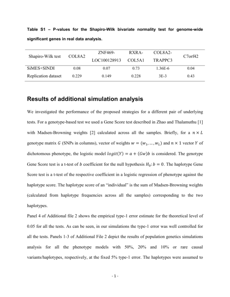
Table S1 – P-values for the Shapiro-Wilk bivariate normality test for genome-wide
significant genes in real data analysis.
Shapiro-Wilk test
COL8A2
ZNF469-
RXRA-
COL8A2-
LOC100128913
COL5A1
TRAPPC3
C7orf42
SiMES+SINDI
0.08
0.07
0.73
1.36E-6
0.04
Replication dataset
0.229
0.149
0.228
3E-3
0.43
Results of additional simulation analysis
We investigated the performance of the proposed strategies for a different pair of underlying
tests. For a genotype-based test we used a Gene Score test described in Zhao and Thalamuthu [1]
with Madsen-Browning weights [2] calculated across all the samples. Briefly, for a 𝑛 × 𝐿
genotype matrix 𝐺 (SNPs in columns), vector of weights 𝑤 = (𝑤1 , … , 𝑤𝐿 ) and 𝑛 × 1 vector 𝑌 of
dichotomous phenotype, the logistic model 𝑙𝑜𝑔𝑖𝑡(𝑌) = 𝑎 + (𝐺𝑤)𝑏 is considered. The genotype
Gene Score test is a t-test of 𝑏 coefficient for the null hypothesis 𝐻0 : 𝑏 = 0. The haplotype Gene
Score test is a t-test of the respective coefficient in a logistic regression of phenotype against the
haplotype score. The haplotype score of an “individual” is the sum of Madsen-Browning weights
(calculated from haplotype frequencies across all the samples) corresponding to the two
haplotypes.
Panel 4 of Additional file 2 shows the empirical type-1 error estimate for the theoretical level of
0.05 for all the tests. As can be seen, in our simulations the type-1 error was well controlled for
all the tests. Panels 1-3 of Additional File 2 depict the results of population genetics simulations
analysis for all the phenotype models with 50%, 20% and 10% or rare causal
variants/haplotypes, respectively, at the fixed 5% type-1 error. The haplotypes were assumed to
-1-
be known without ambiguity. We also performed the same analysis with haplotypes inferred with
Beagle using the reference panel of 1094 individuals to mimic the size of the publicly available
reference panel from the 1000 Genomes Project (www.1000genomes.org) —and the results were
very similar (data not shown). As can be seen from Additional File 2 for genotype scenarios, the
genotype Gene Score test performed better or equally good compared with the haplotype Gene
Score test, whereas for haplotype risk scenarios, the result was the opposite, except for the
“Common” phenotype model. This may be explained by the fact that the frequency of some
common haplotypes may be very high (for example, wild type haplotype); so, if a very common
haplotype is chosen to confer risk, it will be underweighted too much in the haplotype Gene
Score test. Since both Gene Score tests were designed to account for the potential effect of rare
variants or rare haplotype, the relative power of the tests under common disease scenarios may
not follow the expectations. It is also notable that the MinP-val test was on par with the SumPval method for all the phenotype models, except when one of the underlying tests significantly
underperformed the other underlying test. In these cases, MinP-val performed better than SumPval, which is consistent with the conclusions obtained for the different pair of the underlying
tests.
Results of additional real data analysis
In addition to the main genome-wide analysis of the SiMES+SINDI data set, we applied
different pair of underlying tests and our proposed methods to the three regions reported by
Vithana et al. [3]. For the genotype-based test we utilized the regression on principal component
(PC) scores of genotype [4]. To describe the methodology, let us denote 𝐺 as 𝑛 × 𝐿 genotype
matrix, where 𝑛 is the sample size and 𝐿 is the number of SNPs within a region, 𝑌 is 𝑛 × 1
vector of quantitative phenotype, 𝐶 is 𝑛 × 12 matrix of covariates which include age, gender and
-2-
the first ten genotype principal components obtained from Eigenstrat [5]. Further, let us define
the 𝑛 × 𝑝 matrix 𝑃 as a matrix with columns being principal component scores obtained from 𝐺.
The matrix 𝑃 contains the minimum number of principal components with the cumulative
variance no less than 80% of the total variance [4]. In other words, the principal components in
order from highest to lowest variance were recursively added to the matrix 𝑃 until the sum of
variances of the columns exceeded 80% of the total variance (sum of variances of all principal
components). This procedure reduces the number of variables while preserving the major share
of genotype variability. Further, the following regression model was considered:
𝑌 = 𝑎 + 𝑃𝑏1 + 𝐶𝑐 + 𝜀
(1)
where 𝑎 is the constant term, 𝑏 and 𝑐 are 𝑝 × 1 and 12 × 1 vectors of regression coefficients,
and 𝜀 is 𝑛 × 1 vector of error terms. A statistic to test the null hypothesis 𝐻0 : 𝑏1 = 0 is the Fstatistic:
𝐹1 =
(𝑆𝑆𝑅 − 𝑆𝑆𝐹)/𝑝
𝑆𝑆𝐹/(𝑛 − 𝑝 − 13)
(2)
where 𝑆𝑆𝐹 is the sum of squared residuals in the full model (3), and 𝑆𝑆𝑅 is the sum of squared
residuals in the reduced model 𝑌 = 𝑎 + 𝐶𝑐 + 𝜀. Under the null hypothesis the test statistic 𝐹1 is
asymptotically distributed as F random variable with 𝑝 and 𝑛 − 𝑝 − 13 degrees of freedom as
the CCT phenotype is a normally distributed trait [3].
For the haplotype-based test we applied the regression on haplotype clusters obtained from the
affinity propagation algorithm [6]. Clustering of haplotypes is needed to reduce the degrees of
freedom of F-statistic and to overcome the difficulty of analyzing rare haplotypes within a
regression framework. Affinity propagation is a clustering algorithm built on the idea of
exchanging real-valued messages between data points until “a high quality set of exemplars and
-3-
corresponding clusters gradually emerge” [7]. The input of the algorithm requires a similarity
matrix {𝑠(𝑖, 𝑗)}𝑁
𝑖,𝑗=1 , where, for 𝑖 ≠ 𝑗 the element 𝑠(𝑖, 𝑗) is a measure of how well the data point 𝑗
is suited to be an exemplar for the data point 𝑖, and for 𝑖 = 𝑗 the element 𝑠(𝑖, 𝑖) is a measure of
likelihood of the data point 𝑖 to be an exemplar (cluster center). Let us assume we have ℎ unique
haplotypes {𝐻𝑘 , 𝑘 = 1, … , ℎ} for a region (a haplotype 𝐻𝑘 can be written as vector
{𝑥𝑘1 , 𝑥𝑘2 , … , 𝑥𝑘𝐿 }, 𝑥𝑘𝑙 ∈ {0,1}). The order of markers on a haplotype is assumed to be the
physical order on the chromosome. To construct ℎ × ℎ haplotype similarity matrix 𝑠(𝑖, 𝑗) Jin et
al. [6] utilized the following measure:
𝐿
(3)
1
𝑝(𝑥𝑖𝑙 )
𝑠(𝑖, 𝑗) = − ∑
|𝑙𝑜𝑔 (
)| , 𝑖 ≠ 𝑗
𝑝(𝑥𝑗𝑙 )
𝑝(𝑥𝑗𝑙 )
𝑙=1
where 𝑝(𝑥𝑖𝑙 ) = 𝑃(𝑥𝑖𝑙 |𝑥𝑖𝑙−1 ) is the likelihood of the observed allele on the haplotype 𝐻𝑖 on the
place 𝑙 conditional upon the observation of an allele on the place 𝑙 − 1 (this model corresponds
to the first-order Markov chain model suggested by Jin et al. [6]). These probabilities are
estimated using the inferred haplotypes across all the individuals. The elements 𝑠(𝑖, 𝑖) are equal
to the median of values 𝑠(𝑖, 𝑗), 𝑖 ≠ 𝑗, which corresponds to the default setting of the ‘apcluster’
function
in
the
affinity
propagation
R
(www.r-project.org/)
package
“apcluster”
(http://www.psi.toronto.edu/index.php?q=affinity%20propagation). For COL8A2 gene we forced
the algorithm to output two clusters as the initial run gave only one haplotype cluster. Next, let
us assume that all the ℎ haplotypes are split into 𝑘 clusters 𝑆1 , … , 𝑆𝑘 , where we let the cluster 𝑆𝑘
to be the most frequent (assigned to be the reference cluster). The 𝑛 × (𝑘 − 1) regression matrix
𝑛,𝑘−1
𝑅 = {𝑅𝑖𝑗 }𝑖=1,𝑗=1 is constructed as follows: value of 𝑅𝑖𝑗 is the number of haplotypes of 𝑖th
-4-
individual that belong to cluster 𝑆𝑗 . After the construction of 𝑅 matrix the following regression
model is considered:
𝑌 = 𝑎 + 𝑅𝑏2 + 𝐶𝑐 + 𝜀
(4)
where 𝑏2 is (𝑘 − 1) × 1 vector of regression coefficients. The test statistic 𝐹2 for the null
hypothesis 𝐻0 : 𝑏2 = 0 is analogous to (4) where 𝑆𝑆𝐹 is computed for the regression model (6).
The asymptotic distribution of 𝐹2 is F-distribution with 𝑘 − 1 and 𝑛 − (𝑘 − 1) − 13 degrees of
freedom.
The permutations of residuals under the reduced model were applied to estimate the
correlation 𝜌 between the inverse standard normal transforms of theoretical p-values of the
underlying tests. To justify our assumption of bivariate normality we applied the Shapiro-Wilk
test. The corresponding p-values for the three regions are presented in the Table S2. All the pvalues are non-significant at 5% type-1 error which suggests there is no evidence against the
assumption of bivariate normal distribution.
Table S3 shows the theoretical p-values for the described genotype and haplotype tests, for
MinP-val and SumP-val approaches. As can be seen, in spite of haplotype-based test yielding
high p-values, both of the proposed methods performed on par with the genotype-based test. It is
notable that the single-SNP p-values reported by Vithana et al. [3] are more significant than all
the other tests considered. However, gene-based analysis reduces the number of tests from
552318 (genome-wide significance level 9.053E-8) to 36146 —number of genes and betweengene blocks in a data set (genome-wide significance level 1.38E-6), which implies the results
obtained here are also significant on the genome-wide level.
-5-
Table S2 – Additional real data analysis: p-values for the Shapiro-Wilk test.
ZNF469-
ShapiroWilk
COL8A2
LOC100128913
RXRA-COL5A1
0.4938
0.7668
0.6285
bivariate
normality test on (𝑁1∗ , 𝑁2∗ )
Table S3 – Additional real data analysis: the results of the real data analysis and the
single-SNP p-values (SiMES and SINDI meta-analysis) from the original article.
ZNF469COL8A2
LOC100128913
RXRA-COL5A1
Genotype test p-value
2.43E-12
3.65E-12
1.22E-08
Haplotype test p-value
0.9013
9.27E-06
4.05E-05
MinP-val
4.85E-12
7.30E-12
2.45E-08
SumP-val
1.61E-11
4.52E-12
2.34E-09
Single-SNP analysis from
Vithana et al. [3]
rs9938149: 1.63E-16
rs96067: 5.4E-13
rs12447690: 1.92E-14
rs1536478: 3.5E-9
References
1.
Zhao J, Thalamuthu A: Gene-based multiple trait analysis for exome sequencing data.
BMC Proceedings 2011, 5(Suppl 9):S75.
-6-
2.
Madsen BE, Browning SR: A groupwise association test for rare mutations using a
weighted sum statistic. PLoS Genet 2009, 5(2):e1000384.
3.
Vithana EN, Aung T, Khor CC, Cornes BK, Tay W-T, Sim X, Lavanya R, Wu R, Zheng
Y, Hibberd ML et al: Collagen-related genes influence the glaucoma risk factor,
central corneal thickness. Human Molecular Genetics 2011, 20(4):649-658.
4.
Gauderman WJ, Murcray C, Gilliland F, Conti DV: Testing association between disease
and multiple SNPs in a candidate gene. Genetic Epidemiology 2007, 31(5):383-395.
5.
Price AL, Patterson NJ, Plenge RM, Weinblatt ME, Shadick NA, Reich D: Principal
components analysis corrects for stratification in genome-wide association studies.
Nat Genet 2006, 38(8):904-909.
6.
Jin L, Zhu W, Guo J: Genome-wide association studies using haplotype clustering
with a new haplotype similarity. Genetic Epidemiology 2010, 34(6):633-641.
7.
Frey BJ, Dueck D: Clustering by passing messages between data points. Science 2007,
315(5814):972-976.
-7-