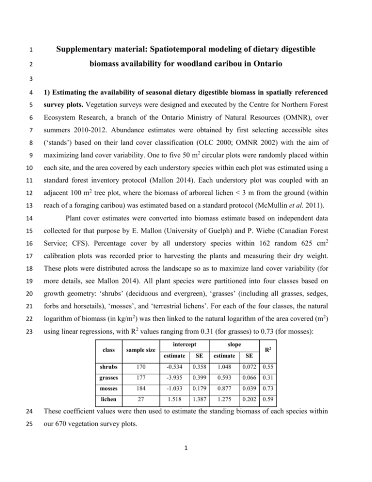
1
Supplementary material: Spatiotemporal modeling of dietary digestible
2
biomass availability for woodland caribou in Ontario
3
4
1) Estimating the availability of seasonal dietary digestible biomass in spatially referenced
5
survey plots. Vegetation surveys were designed and executed by the Centre for Northern Forest
6
Ecosystem Research, a branch of the Ontario Ministry of Natural Resources (OMNR), over
7
summers 2010-2012. Abundance estimates were obtained by first selecting accessible sites
8
(‘stands’) based on their land cover classification (OLC 2000; OMNR 2002) with the aim of
9
maximizing land cover variability. One to five 50 m2 circular plots were randomly placed within
10
each site, and the area covered by each understory species within each plot was estimated using a
11
standard forest inventory protocol (Mallon 2014). Each understory plot was coupled with an
12
adjacent 100 m2 tree plot, where the biomass of arboreal lichen < 3 m from the ground (within
13
reach of a foraging caribou) was estimated based on a standard protocol (McMullin et al. 2011).
14
Plant cover estimates were converted into biomass estimate based on independent data
15
collected for that purpose by E. Mallon (University of Guelph) and P. Wiebe (Canadian Forest
16
Service; CFS). Percentage cover by all understory species within 162 random 625 cm2
17
calibration plots was recorded prior to harvesting the plants and measuring their dry weight.
18
These plots were distributed across the landscape so as to maximize land cover variability (for
19
more details, see Mallon 2014). All plant species were partitioned into four classes based on
20
growth geometry: ‘shrubs’ (deciduous and evergreen), ‘grasses’ (including all grasses, sedges,
21
forbs and horsetails), ‘mosses’, and ‘terrestrial lichens’. For each of the four classes, the natural
22
logarithm of biomass (in kg/m2) was then linked to the natural logarithm of the area covered (m2)
23
using linear regressions, with R2 values ranging from 0.31 (for grasses) to 0.73 (for mosses):
intercept
class
slope
R2
sample size
estimate
SE
estimate
SE
shrubs
170
-0.534
0.358
1.048
0.072
0.55
grasses
177
-3.935
0.399
0.593
0.066
0.31
mosses
184
-1.033
0.179
0.877
0.039
0.73
lichen
27
1.518
1.387
1.275
0.202
0.59
24
These coefficient values were then used to estimate the standing biomass of each species within
25
our 670 vegetation survey plots.
1
26
Next, biomass estimates were converted to digestible biomass estimates. Previously
27
collected biomass samples were used to estimate fractions of Neutral Detergent Fiber (%NDF;
28
including cellulose, hemicellulose and lignin), and Acid Detergent Fiber (%ADF; including only
29
cellulose and lignin), for each species (for methodological details see Mallon 2014). Where
30
possible, fractions were estimated separately for spring (samples taken from May 1st to June
31
15th), summer (June 16th to October 31st) and winter (November 1st to April 31st). Note however
32
that for the majority of species winter samples were never collected and hence summer values
33
were used for both summer and winter. In cases where data at higher taxonomical and/or
34
seasonal resolution were available in the literature, literature values were used (for details see
35
Mallon 2014). Otherwise, missing ADF/NDF values were filled in based on species that were
36
either closely related taxonomically or morphologically similar. To characterize the relationships
37
between ADF, NDF and digestibility, in vitro dry matter digestibility values (IVDMD) over a
38
standard 48 h period were obtained from the published literature on caribou or reindeer for 28
39
plant species together with their respective ADF and NDF values (Mathiesen & Utsi 2000;
40
Storeheier et al. 2002b; a; Ihl & Barboza 2007). Species were again categorized into four classes
41
based on the availability of literature values: shrubs, grasses, mosses and lichens. For the moss
42
group, literature digestibility values (Ihl & Barboza 2007) were coupled with ADF and NDF
43
values from the current study. A linear regression was then fitted within each group to link logit-
44
transformed IVDMD values to logit-transformed ADF, NDF and ΔNDF (the difference between
45
NDF and ADF) values (missing values are due to exclusion in an AIC based model competition):
intercept
class
logit(ADF)
logit(NDF)
logit(NDF-ADF)
sample size
estimate
SE
estimate
SE
estimate
SE
estimate
SE
R2
shrubs
7
-1.295
0.787
-1.647
0.269
-
-
0.349
0.433
0.95
grasses
12
-1.865
0.288
-1.228
0.360
-
-
-1.337
0.515
0.83
mosses
3
1.301
0.568
-
-
-3.168
0.494
-
-
0.95
lichen
6
-1.588
0.494
-0.787
0.178
-
-
-0.346
0.103
0.84
46
47
In combination with our species-specific ADF and NDF fractions, these coefficient values were
48
then used to estimate the available digestible biomass of each species within 670 vegetation
49
survey plots.
50
Finally, to estimate the dietary digestible biomass and nitrogen available to woodland
51
caribou in each plot, we estimated the fraction of each plant species in the diet of woodland
2
52
caribou. To estimate diet composition, GPS radio-telemetry collars equipped with video cameras
53
(Thompson et al. 2013, 2015) were deployed on 15 female woodland caribou across our study
54
area. After the collars were collected, video files were classified according to time of year and
55
the behavior displayed by the animal. Video clips classified as ‘foraging’ were then watched by
56
field assistants well acquainted with boreal flora, and the number of bites taken from each genus
57
of plants was recorded (for further details see Newmaster et al. 2013 and Thompson et al. 2015).
58
The number of bites per genus was then summed across all animals and normalized to yield diet
59
composition for each of three seasons (spring, summer and winter). For each of our survey plots,
60
we then multiplied the digestible biomass and nitrogen content for each species by its fraction in
61
the caribou’s diet before summing all values to yield the total seasonally available dietary
62
digestible biomass and nitrogen per plot:
dietary digestible
biomass (kg/m2)
dietary nitrogen
(kg/m2)
minimum
1st quantile
median
mean
3rd quantile
maximum
spring
2.60E-05
1.59E-03
3.37E-03
2.69E-02
7.26E-03
8.33E-01
summer
1.60E-05
1.25E-03
2.34E-03
1.94E-02
5.59E-03
5.96E-01
winter
3.00E-06
1.45E-03
3.27E-03
3.42E-02
9.18E-03
1.09E+00
spring
4.38E-06
1.51E-04
3.38E-04
1.03E-03
7.97E-04
2.96E-02
summer
1.72E-06
1.06E-04
1.73E-04
6.36E-04
3.02E-04
1.97E-02
winter
1.86E-07
1.00E-04
2.49E-04
1.00E-03
4.88E-04
3.12E-02
63
64
2) Extrapolation of dietary digestible biomass estimates across the landscape. Our final goal
65
was to generate seasonal landscape projections of forage availability, which requires
66
extrapolation of our forage estimates outside of our survey plots. To achieve this objective, we
67
assembled a set of remote-sensed landscape attributes to serve as potential predictors of forage
68
abundance. MODIS-based Normalized Difference Vegetation Index (NDVI; indicative of live
69
green vegetation) values were obtained via the Land Processes Distributed Active Archive
70
Center at the U.S. Geological Survey Earth Resources Observation and Science Center (temporal
71
resolution: 16 days, spatial resolution: 250 m pixels). To create a temporally-independent
72
seasonal NDVI signature, values were averaged over the four core winter months (December-
73
March; herein ‘winter NDVI’) and the four core summer months (June-September; herein
74
‘summer NDVI’) from 2010 to 2013. A digital elevation model (ASTER GDEM; spatial
75
resolution: 25 m pixels) was obtained via NASA’s Reverb (http://reverb.echo.nasa.gov/reverb)
76
and used to generate relative elevation maps by subtracting the DEM value at each pixel from the
3
77
average DEM value within a 500 m radius. Land cover classification (spatial resolution: 30 m
78
pixels) was based on the Ontario Provincial Far North Land Cover map (FNLC v1.3.1, ;OMNR
79
2013). This map does not extend south of ~50° N latitude and so was merged with OLC 2000
80
where necessary. Maps included updated disturbances (fire and harvest) for each year of the
81
study based on data provided by (CFS and OMNR personal).
82
Land cover effects were estimated at two spatial resolutions. The land cover class at each
83
survey plot was taken as the dominant class within 30 m radius of the plot location. Hence, each
84
plot was classified as either: ‘coniferous’ (FNLC 18), ‘lowland’ (a combination of FNLC classes
85
6, 9-14), ‘deciduous’ (FNLC 16), ‘mixed’ (FNLC 17), ‘disturbed’ (FNLC classes 19 and 20), or
86
‘sparse’ (FNLC class 15). However, to avoid singularity, one of these classes had to be omitted
87
from our analysis (here we chose to omit ‘disturbed’). In addition, percent cover for each of
88
seven land cover categories was calculated within a 250 m radius around each of our survey
89
plots. These categories were: ‘coniferous’ (FNLC 18), ‘open lowland’ (FNLC 6, 11 and 13),
90
‘treed lowland’ (FNLC 9, 10, 12 and 14), ‘deciduous lowland’ (FNLC 8 and 25), ‘deciduous’
91
(FNLC 16), ‘mixed’ (FNLC 17), or ‘sparse’ (FNLC class 15). To adjust these percent covers to
92
the area of pristine habitat, values were divided by percent cover of undisturbed land (= 1 -
93
(FNLC1 + FNLC2 + FNLC19 + FNLC20)).
94
As the distribution of total available dietary digestible biomass in our samples is strongly
95
right-skewed, values were log-transformed to reduce heteroscedasticity. Mixed effects models
96
were fitted separately for spring, summer and winter using function lme in R, with site (‘stand’)
97
ID as random effects and a Gaussian spatial residual autocorrelation structure within sites.
98
Initially, all potential explanatory variables were included in the model (summer- and winter-
99
NDVI, relative elevation, and land cover at 30 m and 250 m scales) with no interactions other
100
than quadratic terms for NDVI. Function stepAIC from the R package MASS was then used to
101
find the best combination of predictors based on AIC scores.
102
The best models for each season explained 20-30% of the observed variability in the log-
103
transformed response (10-20% variability explained after back-transformation) but tended to
104
undervalue the magnitude of forage availability, particularly at the high end of the forage
105
availability range. We thus calculated a linear correction factor for each model fit as the slope of
106
a zero-intercept mixed effect model of the back-transformed response variable as function of the
107
back-transformed predictions of the models (fixed effects only).
4
log( available dietary digestible biomass )
winter
spring
summer
MLE
SE
MLE
SE
MLE
SE
Intercept
-37.89500
8.24236
-34.88061
7.04242
-32.52176
6.67173
con_30m
-0.71823
0.27389
-0.71759
0.23475
-0.70305
0.22167
lowland_30m
-0.82212
0.28978
-0.52592
0.24842
-0.70441
0.23449
decid_30m
-1.10116
0.44055
-0.92677
0.37579
-0.83214
0.35665
decid_250m
-1.41566
0.59205
-1.25628
0.50410
-0.98349
0.47931
mixed_250m
-0.79759
0.36730
-0.82425
0.31488
-0.69941
0.29726
NDVI.sum
0.85767
0.23159
0.76863
0.19784
0.69684
0.18746
NDVI.sum^2
-0.00647
0.00160
-0.00566
0.00136
-0.00507
0.00129
NDVI.win
0.28505
0.09273
0.23733
0.07937
0.20585
0.07505
NDVI.win^2
-0.00322
0.00127
-0.00277
0.00109
-0.00238
0.00103
correction factor
6.17424
0.82219
5.01664
0.66776
4.98149
0.65295
108
109
These regression coefficients were then used to generate seasonal maps of expected
110
dietary digestible biomass across the entire study area. Areas covered with water and those
111
disturbed the previous year (for winter and spring), or the current year (for summer), were
112
arbitrarily set to zero.
113
5
114
Supplementary material: Spatiotemporal modeling of wolf density
115
116
The procedure described in the main text allowed us to calculate seven population-level
117
wolf density kernels, four for winter (2009-10 to 2012-13; based on a total of 59,050 GPS points
118
from 32 packs), and three for summer (2010-2012; based on 60,196 GPS points from 34 packs).
119
Local density values (in wolves per km2) across these kernels span three orders of magnitude and
120
ranged from 0.0000661 to 0.271939 (with a mean of 0.006813) in summer and from 0.000202 to
121
0.226921 (with a mean of 0.007418) in winter.
122
A regression analysis of local wolf density (log-transformed) as function of local habitat
123
covariates was then performed separately for summer (with a total of 147,901 hexagonal cells,
124
each 0.22 km2 in area) and winter (with a total of 169,738 hexagonal cells). Each hexagonal cell
125
associated with a wolf density value was characterized by temporally-matched values of multiple
126
remote-sensed landscape covariates that were used to predict local wolf density. These included
127
seasonal NDVI, relative elevation, and FNLC v1.3.1 land cover classes (see the above forage
128
modelling section for more details). Cells were also characterized based on their proximity to
129
dumps and settlement (if < 1 km, 1, otherwise, 0), their proximity to roads (if < 500 km, 1,
130
otherwise, 0), and their distance to shoreline of rivers or large lakes. Land cover classes were
131
amalgamated into 9 categories: water (open and turbid classes), open lowland (open fen, open
132
bog, and freshwater marsh classes), treed lowland (treed peatland, treed fen, treed bog, and
133
coniferous swamp classes), deciduous lowland (thicket swamp and deciduous swamp classes),
134
deciduous upland (deciduous treed class), mixed upland (25-75% deciduous, 25-75% coniferous,
135
and mixed treed class), sparse forest (sparse treed class), disturbed (disturbed treed/shrub and
136
disturbed non/sparse classes; representing natural and anthropogenic disturbances), and newly
137
disturbed (< 1 year from fire or forestry disturbance). The coniferous treed class was withheld
138
from the analysis and thus served as a reference class for the resulting inference.
139
Generalized least squares regression models were fitted using function gls in the R
140
package nlme, which allowed explicitly accounting for spatial autocorrelation in the response
141
variable. For each season, model fits were repeated 50 times, each based on a different sample
142
consisting of 2% of the total available data and taken at regular spatial intervals. Averaging the
143
resulting 50 values for each coefficient allowed us to obtain robust coefficient estimates despite
144
the inherent spatial autocorrelation in the data (for further details see Kittle et al. submitted MS).
6
145
Log(wolf density)
SUMMER
WINTER
Average β
Average SE
Average β
Average SE
Intercept
-7.867193
0.340019
-7.221411
0.229412
le500m
-0.000745
0.004297
-0.002081
0.004348
NDVI
0.006325
0.004431
-0.011382
0.002852
NDVI_last
-0.001173
0.003000
0.002686
0.002218
dump
0.790474
0.502683
0.872039
0.471592
settle
-0.161816
0.543381
-0.080476
0.442302
prime500
0.100127
0.081268
0.024167
0.086373
sec500
0.140625
0.051471
0.046516
0.055456
distshore_km
-0.189199
0.050909
-0.111469
0.052324
water
0.121834
0.131908
-0.151999
0.118354
open_low
-0.012386
0.161552
-0.431312
0.175744
treed_low
-0.029356
0.082822
-0.126191
0.086712
decid_low
0.163702
0.571260
-0.035573
0.592419
lcV16 (decid)
0.163390
0.180313
0.368103
0.182048
lcV17 (mix)
0.095694
0.125011
0.256256
0.133332
lcv15 (sparse)
0.051991
0.291906
-0.043764
0.306415
disturb
0.153453
0.084417
0.060398
0.087992
disturb_new
0.005035
0.297817
-0.155916
0.275190
146
147
The pseudo R2, based on regressing the all observed wolf density values against the averaged
148
model’s predictions, was low (~ 5%), and the linear correlation between predicted and observed
149
was app 0.2. These goodness-fit values indicate a poor model fit and reflect the week links
150
between local wolf density and remote-sensed habitat attributes in our study area. Averaged
151
regression coefficients were then used to project wolf density maps across the entire study area
152
for each season-year combination.
153
7
154
Supplementary material: Spatiotemporal modeling of moose habitat
155
156
Moose occupancy was obtained from fixed-wing aerial surveys flown from Feb. 13 to
157
Mar. 12, 2011 in the extreme northwest of our study area, and Jan. 5 to Mar. 5, 2012 in the
158
extreme southeast of our study area. Both surveys covered roughly 22,500 km2. 1 km transects
159
oriented north-to-south were placed systematically across both landscapes at 5 km intervals to
160
encompass anticipated gradients in disturbance and wolf density. Two observers searched within
161
500 m on either side of the aircraft and recorded the GPS position as well as the number, age,
162
and sex of detected moose. Overall, 4322 km were flown in the northwest survey, with 72 moose
163
sited, and 4236 km were flown in the southeast survey, with 98 moose sited.
164
We identified landscape covariates of biological relevance to moose from land cover,
165
productivity, and weather data. We used FNLC v1.3.1 at a 30 m resolution, modified as
166
described above, to classify forest cover. Because remotely sensed data are inherently error
167
prone, we calculated the difference in mean seasonal NDVI (∆NDVI) for each buffer, estimated
168
as described above, as a correction for available deciduous foliage (i.e., prime moose foraging
169
habitat). We calculated mean snow depth (based on the projection described below) because
170
deeper snow inhibits moose movement and increases vulnerability to predation. Because relative
171
elevation influences dominant vegetation types at a fine scale (i.e., highlands vs. lowlands), we
172
calculated relative elevation within 500 m of a buffer centroid based on digital elevation models
173
from NASA’s Reverb database. We placed circular (250 m radius) buffers around each moose
174
location and characterized landscape covariates within these buffers as proportional coverage for
175
categorical variables (i.e., land cover classes), and as mean values for continuous variables (i.e.,
176
snow depth). We created non-overlapping unused buffers spaced at 600 m between centroids
177
along the flight path and similarly calculated landscape covariates within each. In total, we
178
recorded 98 used vs 5997 unused locations in the southeast survey, and 72 used and 6618 unused
179
locations in the northwest survey.
180
We estimated the probability of moose habitat use using logistic regression, per the
181
resource selection function (RSFs) methodology described by Manly et al. (2002). We have
182
excluded deciduous habitat from the model to eliminate perfect collinearity between categorical
183
stand types. Thus selection for stand types represents selection relative to deciduous habitat. To
184
account for any effects of the survey year (the southeast survey was performed one year after the
8
185
northwest surveys), we included the survey identity as a main effect in the RSF (southeast = 0,
186
northwest = 1). We reduced the full model using stepwise AIC and the final model had a
187
Nagelkerke's pseudo R2 of 0.15:
MLE
SE
Intercept
-6.97007
0.66988
∆NDVI
0.11326
0.01375
Relative elevation (m)
--
--
Snow depth (m)
-0.01362
0.00677
Water
-2.95998
0.48004
Lowland
-1.90219
0.33182
Mixed
--
--
Conifer
-2.25297
0.39014
Sparse
-3.47724
1.96844
Disturbance
--
--
Recent burn
--
--
Survey
0.33583
0.18111
188
189
For the purpose of predicting across the entire landscape, the ‘Survey’ effect was
190
averaged (halved) and added to the ‘Intercept’. The resulting logistic model was used to project
191
moose relative probability of use for each 0.22 km2 hexagonal cell across the study area.
9
192
Supplementary Material: Spatiotemporal modeling of snow depth in Ontario
193
194
Observed snow depth data was collected by P. Wiebe (Canadian Forest Service) between
195
2011 and 2013 at several locations across the greater study area, using two methods: fixed
196
cameras that capture daily photos of snow level throughout the winter at the same site, and
197
transects that provides snow depth measurements across different landcover types but with little
198
temporal replication. Combined, these two methods yielded 2326 snow depth observations that
199
could be coupled with spatiotemporal predictors.
200
Each observation was matched with two spatiotemporal predictors; the closest (in space
201
and time) NOAA snow depth value (temporal resolution: 3 hr, spatial resolution: 40 km pixels;
202
NARR dataset DSI-6175), and the closest NDVI value (temporal resolution: 16 days, spatial
203
resolution: 250 m pixels; Land Processes Distributed Active Archive Center). In addition, each
204
sampling location was matched with several spatial covariates. To create a temporally-
205
independent seasonal NDVI signature, values were averaged over the four core winter months
206
(December-March; hereon ‘winter NDVI’) and the four core summer months (June-September;
207
hereon ‘summer NDVI’) for each observation year. A digital elevation model (ASTER GDEM;
208
spatial
209
(http://reverb.echo.nasa.gov/reverb) and used to generate relative elevation maps by subtracting
210
the DEM value at each pixel from the average DEM value within a 500 m radius. Land cover
211
classification (spatial resolution: 30 m pixels) were based on the Ontario Provincial Far North
212
Land Cover Database (FNLC v1.3.1). Each sampling location was classified as either ‘water’
213
(FNLC 1 or 2), ‘treeless’ (FNLC 6, 11, 13, 21 or 22), ‘deciduous’ (FNLC 8, 25, 16 or 17),
214
‘sparse’ (FNLC class 9, 10, 12, 14, 15, 19 or 20), ‘coniferous’ (FNLC 18), or ‘road’ (including
215
hydro corridors).
resolution:
25
m
pixels)
was
obtained
via
NASA’s
Reverb
216
Model fitting was performed in two stages to appropriately account for the structure of
217
the data set. First, a spatiotemporal mixed effects model was fitted using function lme in R
218
(package nlme) with the natural logarithm of the observed snow depth as the response variable,
219
the natural logarithm of the NOAA snow depth and the NDVI value as the predictors, and the
220
sampling location as random effect. In the second stage, site effects were modeled as function of
221
all spatial covariates (including interactions between seasonal NDVI, relative elevation and
222
landcover), while controlling for sampling method (transect vs. camera), using function gls with
10
223
Gaussian spatial autocorrelation structure. This full model was then reduced based on BIC
224
competition using function stepAIC (package MASS in R). The final model explains 45% in the
225
variation in site effects. Combined, the resulting coefficient estimates explain more than 88% of
226
the observed variability in snow depth measurements across space and time:
main
effects
site
effects
log( snow depth)
MLE
SE
Intercept
3.20034
0.10079
log(NOAA snow depth + 1)
0.44718
0.01487
NDVI
-0.02502
0.00155
Intercept
0.05139
0.02005
Road
-0.14147
0.05741
Water
-0.35965
0.05381
Relative Elevation * coniferous
-0.01877
0.00609
Relative Elevation * deciduous
-0.01313
0.00504
Relative Elevation * sparse
-0.01693
0.00576
Relative Elevation * winter NDVI
0.00038
0.00010
227
228
11
229
Supplementary material: posterior coefficient estimates
230
caribou ID
1.102
1.112
1.113
1.123
1.130
1.135
1.136
1.141
1.148
1.201
1.202
1.203
2.152
2.155
2.256
2.259
2.261
2.262
2.263
2.268
2.276
2.279
2.280
2.281
2.283
2.284
2.296
2.297
2.313
2.314
θ0
θs
0.011
0.011
0.012
0.011
0.014
0.012
0.014
0.011
0.014
0.009
0.010
0.009
0.014
0.011
0.014
0.010
0.013
0.008
0.016
0.014
0.009
0.011
0.011
0.011
0.013
0.014
0.013
0.010
0.010
0.010
0.000
0.000
0.010
0.008
0.000
0.000
0.000
0.000
0.000
0.006
0.012
0.008
0.000
0.009
0.016
0.000
0.014
0.015
0.000
0.000
0.008
0.000
0.006
0.000
0.017
0.000
0.000
0.017
0.000
0.000
median posterior coefficient values
selection
α
β
DDB wolf density moose habitat
0.005 0.000 1.893
-9.612
-0.345
0.047 0.000 2.755
3.276
-39.030
0.055 0.000 -0.408
-17.106
-0.610
0.004 0.000 2.843
-8.324
-4.255
0.085 0.000 1.238
-11.079
-9.583
0.005 0.017 2.263
-2.392
-0.131
0.202 0.000 2.540
-5.149
5.391
0.029 0.000 1.850
-5.420
-3.102
0.161 0.000 -2.642
0.285
-0.246
0.032 0.000 3.619
-5.390
-8.382
0.004 0.000 2.361
-5.236
-0.359
0.002 0.000 1.286
-2.399
-2.041
0.008 0.000 1.949
15.162
-0.933
0.250 0.000 0.915
-14.583
-0.074
0.163 0.000 -3.324
0.085
-4.492
0.016 0.000 6.503
-0.743
-35.609
0.005 0.004 4.552
6.439
-3.561
0.025 0.000 -1.187
-17.931
-3.202
0.009 0.000 2.567
6.952
-10.673
0.037 0.000 2.464
-10.530
-0.456
0.027 0.000 1.465
-16.544
-8.601
0.096 0.000 -1.506
-2.419
-24.347
0.026 0.000 3.301
-8.079
-6.984
0.075 0.000 1.470
-1.376
-8.426
0.040 0.000 0.036
-0.433
-31.024
0.065 0.000 -2.400
-0.184
-9.466
0.009 0.000 3.360
5.592
-0.224
0.019 0.000 0.934
-12.376
-4.826
0.040 0.000 5.050
-7.308
0.221
0.027 0.000 5.821
0.149
-0.225
231
232
12
233
Supplementary material: Bibliography
234
235
Ihl, C. & Barboza, P.S. (2007) Nutritional value of moss for arctic ruminants: a test with
muskoxen. Journal of Wildlife Management, 71, 752–758.
236
237
238
239
Kittle, A., Patterson, B., Anderson, M., Moffatt, S., Rodgers, A., Shuter, J., Reid, D., Baker, J.,
Brown, G., Thompson, I., Street, G., Avgar, T., Hagens, J., Iwachewski, E. & Fryxell, J.
Wolves adapt territory size, not pack size to local habitat quality. Journal of Animal
Ecology, submitted MS.
240
241
242
Mallon, E.E. (2014) Effects of Disturbance and Landscape Position on Vegetation Structure and
Productivity in Ontario Boreal Forests: Implications for Woodland Caribou (Rangifer
Tarandus Caribou) Forage. University of Guelph.
243
244
Mathiesen, S.D. & Utsi, T.H.A. (2000) The quality of the forage eaten by Norwegian reindeer on
South Georgia in summer. Rangifer, 20, 17–24.
245
246
247
McMullin, R.T., Thompson, I.D., Lacey, B.W. & Newmaster, S.G. (2011) Estimating the
biomass of woodland caribou forage lichens. Canadian Journal of Forest Research, 1969,
1961–1969.
248
249
250
251
Newmaster, S.G., Thompson, I.D., Steeves, R.A.D., Rodgers, A.R., Fazekas, A.J., Maloles, J.R.,
Mcmullin, R.T. & Fryxell, J.M. (2013) Examination of two new technologies to assess the
diet of woodland caribou : video recorders attached to collars and DNA barcoding.
Canadian Journal of Forest Research, 900, 897–900.
252
OMNR. (2002) Ontario Land Cover Classification.
253
OMNR. (2013) Ontario Provincial Far North Land Cover v1.3.1.
254
255
Storeheier, P., Mathiesen, S., Tyler, N. & Olsen, M. (2002a) Nutritive value of terricolous
lichens for reindeer in winter. Rangifer, 34, 247–257.
256
257
258
Storeheier, P., Mathiesen, S., Tyler, N., Schjelderup, I. & Olsen, M. (2002b) Utilization of
nitrogen-and mineral-rich vascular forage plants by reindeer in winter. Journal of
Agricultural Sciences, 139, 151–160.
259
260
261
Thompson, I.D., Wiebe, P., Mallon, E., Rodgers, A.R., Fryxell, J.M., Baker, J. & Reid, D. (2015)
Factors influencing the seasonal diet selection by woodland caribou in boreal forests in
Ontario. Canadian Journal of Zoology, in press.
262
13