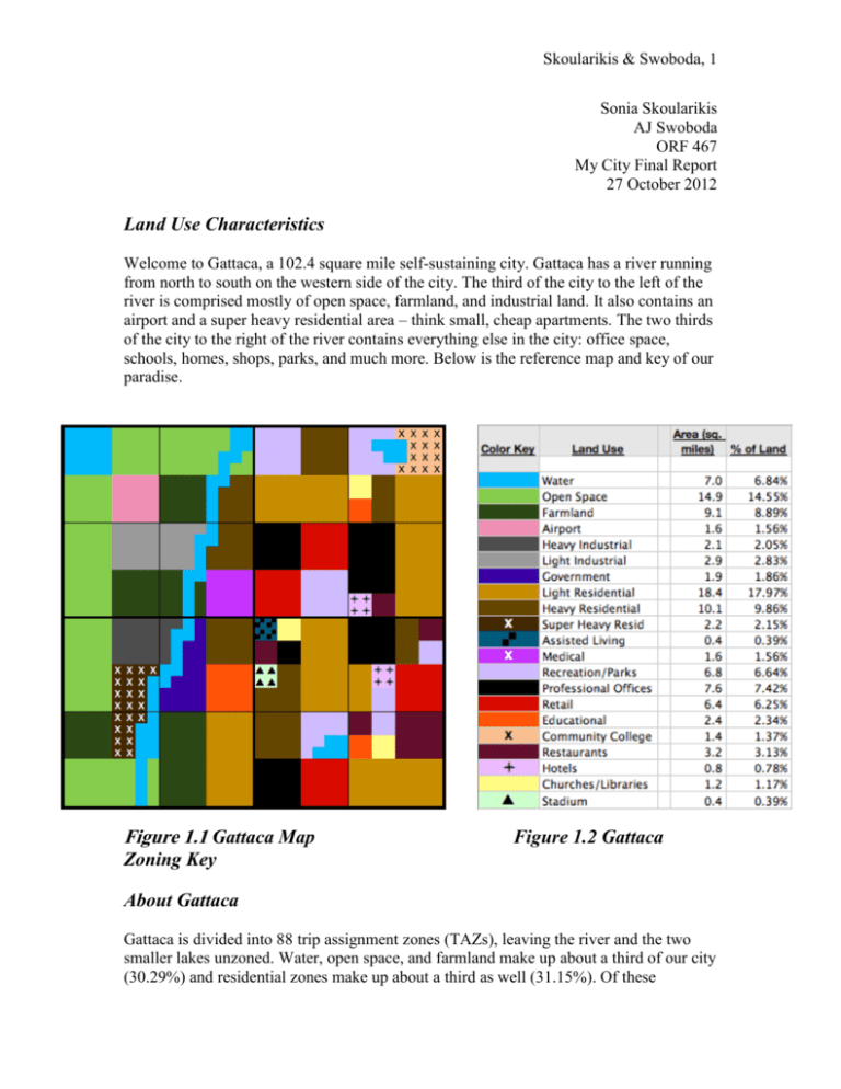
Skoularikis & Swoboda, 1
Sonia Skoularikis
AJ Swoboda
ORF 467
My City Final Report
27 October 2012
Land Use Characteristics
Welcome to Gattaca, a 102.4 square mile self-sustaining city. Gattaca has a river running
from north to south on the western side of the city. The third of the city to the left of the
river is comprised mostly of open space, farmland, and industrial land. It also contains an
airport and a super heavy residential area – think small, cheap apartments. The two thirds
of the city to the right of the river contains everything else in the city: office space,
schools, homes, shops, parks, and much more. Below is the reference map and key of our
paradise.
Figure 1.1 Gattaca Map
Figure 1.2 Gattaca
Zoning Key
About Gattaca
Gattaca is divided into 88 trip assignment zones (TAZs), leaving the river and the two
smaller lakes unzoned. Water, open space, and farmland make up about a third of our city
(30.29%) and residential zones make up about a third as well (31.15%). Of these
Skoularikis & Swoboda, 2
residential zones, 57.69% is light residential, 31.65% is heavy residential, 6.90% is super
heavy residential. Other residential zones such as assisted living and hotels make up the
rest.
Throughout the eastern two thirds of the city, light residential and heavy residential are
scattered fairly evenly, with light residential – think rural and suburban housing – being
more on the outskirts of the city. The super heavy residential zones were placed alongside
the industrial workplace zones, on the western side of the river, as it was concluded that
many of the factory workers of the city would need cheap, affordable housing.
For the most part, each chunk of light and heavy residential zones would have parks and
recreation, retail, restaurants, office space, and a school as nearby as possible. This
created more of a “neighborhood” feel where not all families would have to travel across
the city on a daily basis. Of our parks and recreation category, the zones that surround the
two lakes in the northeastern and southeastern corners of the city are simply parks.
Whereas the zones that are more in the heart of the city consist of playing fields and other
recreational facilities.
The hospital was placed in the center of the city in order to minimize the amount of
distance required for travel in case of an emergency at any location in the city. The
assisted living facility was placed adjacent to the hospital since it was concluded that the
elderly would frequent the medical facilities more than others.
Demographics
The 2010 US Census data reported that the average household size has declined from
2.62 in 2000 to 2.59 in 2010 – reason for this being partly due to the increase of more
single-person households. Therefore Gattaca has been designed to have roughly as much
land space dedicated to light residential as it does to heavy and super heavy residential in
order to accommodate more, smaller sized households.
Included below are two breakdowns of the overall city population and the overall student
population.
Figure 1.3 Gattaca Pop. Breakdown
Figure 1.4 Gattaca Student Breakdown
Skoularikis & Swoboda, 3
As shown in Figure 1.3, 20% of Gattaca’s population is made up of children, defined by
the age range 0-18 years. These children, as shown in Figure 1.4, are divided amongst
elementary, middle, high school, and private (K-12) school. Community college students
make up roughly three percent of the total population. Since this is a community college,
unlike university students, these students do not live within the confines of the college.
Roughly 8.4% of Gattaca is unemployed, a rate obviously higher than what a city should
strive for, but this high unemployment rate has been attributed to the recent global
recession and has been steadily decreasing. The elderly population – defined as 65 years
of age and older – makes up 23% of the city’s total population. These people, though of
course not all living at an assisted living facility, have chosen to retire in order to explore
and enjoy other parts of life.
Figure 1.5 Breakdown of Different Types of Employment
Workers in Gattaca make up about 45.55% of the total population. As shown above, this
count includes jobs at all types of places – professional offices, industrial workplaces,
restaurants, retail, medical, governmental, etc. The “density” column in the table above
refers to the amount of workers per square mile while the number of employees was
calculated by multiplying the density by the actual area of the category of work in
Gattaca.
Although not included in Figure 1.1, some form of a transportation network is required
for the inhabitants of the city to go about living – people go to work, school, parks,
restaurants, shops, the airport, and more. Since we did not design a network of streets and
Skoularikis & Swoboda, 4
highways, we have estimated all of the trip lengths of our inhabitants by multiplying the
distance between zones by a factor of 1.2 – this factor accounts for the added distance
travelled during a trip due to the meandering of roads.
Demand for Transportation
Trip Generation
Production and Attraction vectors were created for each of the nine
different types of trips that a citizen of Gattaca could take in the city.
These trips are: home to work, home to school, home to other, work to
home, school to home, other to home, work to other, school to other, and
finally other to other.
For the Home -> Work trips, the production vector (‘P’) comes from the
vector labeled ‘# of Workers Living at Category’, which represents the
number of workers living in each of the zones (i.e. Super Heavy
Residential, Heavy Residential, and Light Residential). The attraction
vector (‘A’) is created from the ‘Employees Working at Category’ vector,
which distributes the workers into different zones, which offer jobs based
on the density of each workplace.
For Home -> School, ‘P’ came from the sum of the ‘# of School Age
Children’ vector and the ‘University Students’ vector. The ‘A’ came
directly from the ‘School Enrollment’ vector.
For Home -> Other, the ‘P’ is a scaled version of the vector titled ‘People
Possibly Going from Home to Other’. This vector gives 80% of the sum of
‘# of Workers Living at Category’, ‘# of School-Age Children’, and
‘University Students’, plus the ‘Unemployed and Elderly’. In this manner,
we account for the 80% of workers and students who return home after
work and school, respectively, who may leave home again. We also
account, as well, for the unemployed and elderly who are assumed to have
not left in the first place. The scaling factor is approximately 0.722, and is
calculated by dividing the total of the ‘People Possibly Going from Home
to Other’ by the total number of people who could go from home to other
(total # of people who could go Home -> Other = Work -> Home trips +
School -> Home trips + (250,000 - Home to Work trips - Home to School
trips)). The ‘A’ is a scaled version of the ‘Other Attraction’ vector. This
vector is the sum of the ‘Retail Floor Space (# of patrons/day)’, the
Skoularikis & Swoboda, 5
‘Restaurant Floor Space’, and the ‘Recreation (# of patrons per day)’
vectors. Therefore it gives positive values for zones such as
recreation/parks, the stadium, retail, etc.
The Work -> Home (School -> Home) ‘P’ vector is merely 80% of the
attraction vector for the Home -> Work (Home -> School) trips. Similarly,
the ‘A’ vector is 80% of the production vector for Home -> Work (Home > School) trips.
Other -> Home trips have a ‘P’ that is a scaled version of the ‘Other
Attraction’ vector. ‘A’ is a scaled version of the ‘Res. Pop’ vector.
For Work -> Other, the ‘P’ vector is 20% of the attraction vector of Home
-> Work since 20% of the workers go to other (rather than returning
directly home) after work. The ‘A’ vector is again a scaled version of the
‘Other Attraction’ vector.
For School -> Other, the ‘P’ vector is 20% of the attraction vector of
Home -> School since 20% of the students go to other (rather than
returning directly home) after school. The ‘A’ vector, like the ‘A’ vector
for Home -> Work trips, is a scaled version of the ‘Other Attraction’
vector.
For Other -> Other trips, the production and attraction vectors are equal
and were calculated by scaling the ‘Other Attraction’ vector. Figure 2.1
shows the first and last several entries of all ‘P’ and desired ‘A’ vectors by
trip type as well as the total number of trips at the bottom. Figure 2.2
summarizes the scaling factor, if any, for each of the production and
attraction vectors, also organized by trip type.
Figure 2.1 Shortened [P] and [A] Vectors by Trip Type
Skoularikis & Swoboda, 6
Figure 2.2 Scaling factors of [P] and [A] Vectors by Trip Type
Trip Type
[P] Scaling
[A] Scaling
Factor
Factor
Home to Work
1.000
1.000
Home to
1.000
1.000
Home to Other 0.722
0.552
Work to Home
0.800
0.800
School to
0.800
0.800
Other to Home 0.674
0.760
0.200
0.081
School to Other 0.200
0.041
1.105
1.105
School
Home
Work to Other
Other to Other
The trips are divided into four different groupings: Home, Work, School,
and Other.
The first three categories are more or less self-explanatory, The Home ->
Work trip type represents employees leaving for work in the morning. The
Home -> School trip type accounts for (grade school, high school, and
elementary school) going to class in the morning. Home -> Other trips
could be trips made by elderly or unemployed individuals who run errands
or leave the house at any time of the day; alternatively the trips can
represent workers and students who are leaving home again after
returning from work or school respectively.
Skoularikis & Swoboda, 7
Work -> Home trips represent 80% of the workforce returning directly
home after work in the evening. Similarly, School -> Home trips stand for
80% of the students returning directly home from school after classes end
in the afternoon. The Other -> Home trip type accounts for all the people
who must return home after coming out to run errands, go to restaurants,
etc.
Work -> Other trips represent the remaining 20% of the workforce who go
directly to a destination other than home after business hours.
Correspondingly, the School -> Other trips show the 20% of students who
make trips after school to places other than home. Finally, the Other ->
Other trips include any number of possibilities, for instance going from a
restaurant to the stadium. This trip type could occur during any part of the
day.
Figure 2.3 summarizes the total number of trips for each trip type as well
as the final total number of trips made. The total values in Figure 2.3 were
calculated in the following manner, based on the assumption that each
person makes an average of four trips per day. Since the population of
Gattaca is 250,000 individuals, this meant we needed the total number of
trips for all of the 9 trip types to sum up to 1,000,000.
The number of Home to Work trips is equal to the number of workers in
the city, 113,870. Similarly, the number of Home to School trips equals the
number of students in the city, 155,675.
The Work (School) to Home number is merely 80% of the Home to Work
(School) value. The Work (School) to Other number is 20% of the Home
to Work (School) value.
The remaining values, Home to Other, Other to Home, and Other to Other
must sum up to 657,000 (the result of 1,000,000 minus the values for all
other trip types). We operated under the assumption that the number of
Home to Other trips (x) should be 50% of the number of Other to Other
trips (2x). Then the number of Other to Home trips should be 657,000 - 3x.
An additional assumption is that everyone who goes out must then return
home later in the day. As a direct result, the sum of the Home to Other,
Work to Other, and School to Other trips must equal the number of Other
to Home trips. In mathematical terms, x + 22,774 + 11,526 = 657,000 - 3x.
Skoularikis & Swoboda, 8
Solving for x, we find that the number of Home to Other trips is 155,675,
meaning that the number of Other to Other trips is 2*155,675 = 311,350.
Subtracting to get the number of Other to Home trips gives 189,975.
Figure 2.4 gives the comparison table information submitted along with
Assignment 2b.
Figure 2.3 Trip Totals by Trip Type
Production and
Attractions
Summary
Home to Work
113,870
Home to School
57,630
Home to Other
155,675
Work to Home
91,096
School to Home
46,104
Other to Home
189,975
Work to Other
22,774
School to Other
11,526
Other to Other 311350
TOTAL TRIPS:
Figure 2.4 MyCity Comparisons
Trip Distribution
1,000,000
Skoularikis & Swoboda, 9
The process used to generate the Trip arrays is based on the Gravity
Model, as depicted in Figure 2.5. In the below equation Tij is the i, jth entry
of the Trip array. As suggested in class, we assumed that K was equal to
the identity matrix. The A’s and P’s are specified by the attraction and
production vectors, based on trip type, as described in the beginning of the
Trip Generation section.
To calculate the distance matrix, we used the Cartesian distance for
interzonal distances. For all trip types with the exception of Other to
Other, for intrazonal distances, we used 50% of the square root of the area
of the zone. For Other to Other, we multiplied each of these intrazonal
distances by 100 to reduce the incentive for intrazonal trips.
For all standard trip types, from this distance matrix, we calculated the F
matrix by taking Fij = 1/Dij2. The Home to Work (inv D) and Home to
Work (inv sqrt D) used an alternative F matrix, calculated by Fij = 1/Dij
and Fij = 1/SQRT(Dij), respectively. The only other modification made to
these calculations was to iterate the process with an altered ‘A’ vector
calculated by Anew = Adesired*Ainput/Aoutput,previous, while concurrently
calculating the error. Iterating the process until error terms fall below 1%
each results in an approximate Trip array for a given category of trip (ex:
Home -> Work).
Figure 2.5 The Gravity Model
The Trip arrays for each of the different nine trip types can be found in
the corresponding excel documents. Figure 2.6, however, shows a small
portion of a sample Trip array for Home -> Work trips.
Skoularikis & Swoboda, 10
Figure 2.6 Subset of the Home -> Work Trip Array
Skoularikis & Swoboda, 11
Shown below, in Figure 2.7 and Figure 2.8, are two tables describing the
trip lengths of the different types of trips.
Figure 2.7 gives a brief summary that shows the average trip length
distance for nine trip types – the six unique types of trips from the initial
nine, followed by the Home -> Work trips generated with different F
matrices.
Figure 2.8 shows a mile-by-mile breakdown of the six unique types of
trips. We used the data in this table to create our CDF graphs on the
following pages.
Figure 2.7 Average Trip Lengths
Figure 2.8 Mile-by-Mile Breakdown of Trips
Miles/Trip
1.00
H->W
0.03
H->S
1.15
H->O
-
W->O
0.04
O->O
0.00
S->O
-
Skoularikis & Swoboda, 12
2.00
3.00
4.00
5.00
6.00
7.00
8.00
9.00
10.00
11.00
12.00
13.00
14.00
15.00
16.00
17.00
18.00
19.00
20.00
21.00
22.00
23.00
24.00
25.00
26.00
27.00
30.00
31.00
32.00
33.00
53.00
58.00
64.00
0.09
10.35
21.47
32.78
48.92
60.65
74.37
80.05
86.35
90.77
94.11
94.72
94.96
95.10
95.66
95.77
97.66
98.57
98.81
99.06
99.07
99.22
99.22
99.41
99.41
99.45
99.55
99.97
99.97
100.00
100.00
100.00
100.00
1.42
7.09
9.15
16.27
29.76
32.89
53.37
56.77
71.72
85.09
88.35
88.67
88.71
88.71
88.71
88.71
97.07
97.44
97.44
97.44
98.71
98.71
99.31
100.00
100.00
100.00
100.00
100.00
100.00
100.00
100.00
100.00
100.00
0.04
0.62
3.80
6.41
12.40
18.94
26.72
35.39
46.52
55.76
58.51
59.16
59.90
62.35
62.88
64.93
65.03
65.09
66.11
71.35
71.86
76.25
76.35
78.69
78.71
78.84
82.95
98.24
98.24
99.24
99.24
99.24
99.24
0.64
3.51
4.36
10.00
23.41
26.70
35.97
48.10
59.03
83.92
93.77
94.50
94.52
94.84
94.84
96.93
97.20
98.35
98.56
98.91
98.98
99.23
99.49
99.93
99.93
99.93
99.93
99.93
99.93
99.93
99.93
99.93
99.93
0.00
5.48
7.36
8.87
26.44
38.66
63.44
69.61
69.92
70.11
87.79
88.09
89.16
89.16
94.89
95.21
95.22
96.91
96.91
96.91
96.91
96.91
96.91
96.91
96.91
96.91
96.91
96.91
97.04
97.04
97.04
97.04
100.00
1.90
3.50
5.68
12.96
16.80
47.93
50.14
58.01
71.35
71.48
73.54
73.72
80.50
80.50
82.41
82.42
82.42
82.42
89.58
98.08
100.00
100.00
100.00
100.00
100.00
100.00
100.00
100.00
100.00
100.00
100.00
100.00
100.00
Skoularikis & Swoboda, 13
Home Based Work
1.00
0.90
% of Total Miles
0.80
0.70
0.60
0.50
0.40
0.30
0.20
0.10
0.00
0.00
5.00
10.00
15.00
20.00
25.00
30.00
35.00
Miles per Trip
Home Based School
1.00
0.90
% of Total Miles
0.80
0.70
0.60
0.50
0.40
0.30
0.20
0.10
-
5.00
10.00
15.00
Miles per Trip
20.00
25.00
30.00
Skoularikis & Swoboda, 14
Home Based Other
1.00
0.80
% of Total Miles
0.60
0.40
0.20
-
5.00
10.00
(0.20)
15.00
20.00
25.00
30.00
35.00
Miles per Trip
Work Based Other
1.00
0.90
% of Total Miles
0.80
0.70
0.60
0.50
0.40
0.30
0.20
0.10
-
5.00
10.00
15.00
Miles per Trip
20.00
25.00
30.00
Skoularikis & Swoboda, 15
School Based Other
1.00
0.90
0.80
% of Total Miles
0.70
0.60
0.50
0.40
0.30
0.20
0.10
-
5.00
10.00
15.00
Miles per Trip
20.00
25.00
Skoularikis & Swoboda, 16
Other Based Other
1.00
0.90
0.80
% of Total Miles
0.70
0.60
0.50
0.40
0.30
0.20
0.10
-
10.00
20.00
30.00
40.00
50.00
60.00
70.00
Miles per Trip
The following two graphs depict the CDF curves of all six unique trip types. The first
graph includes all distances of trips – some of our trips had a distance of up to 64 miles –
while the second graph is constrained to the range from zero to 15 miles.
Skoularikis & Swoboda, 17
CDF: 6 Different Trip Types
100.00
90.00
80.00
% of Total Trips
70.00
H->W
60.00
H->S
50.00
H->O
40.00
W->O
30.00
O->O
S->O
20.00
10.00
-
10.00
20.00
30.00
40.00
Miles per Trip
50.00
60.00
70.00
The steepest line out of the six trip types is the Home to Work trips. This type peaks the
fastest because we planned the city so that people lived conveniently near where they
worked. The proximity between homes and workplaces meant that a greater amount of
shorter trips occurred for Home to Work trips as opposed to other trip types. The least
steep line is the Home to Other trips. This indicates that zones involving 'Other'
attractions are inconveniently located compared to where people generally live.
Skoularikis & Swoboda, 18
CDF: 6 Different Trip Types
100.00
90.00
80.00
% of Total Trips
70.00
H->W
60.00
H->S
50.00
H->O
40.00
W->O
30.00
O->O
S->O
20.00
10.00
-
2.00
4.00
6.00
8.00 10.00
Miles per Trip
12.00
14.00
16.00
This graph displays the x-range from 0 to 15, the interval on which the CDFs vary most
and thus the area of interest for analysis. However, our trip types involve trips that go up
to 64 miles long. The reason for these extremely long trips is the modification to the
distance matrix for the Other to Other trip type. For this type of trip, we multiplied each
entry on the diagonal of the distance matrix by 100 in order to decrease the likelihood
that people would make intrazonal, Other to Other trips. Yet this penalty resulted in an
extremely small percentage of trips that were very long (30 to 60 miles per trip).
Person Trip Length Distribution Analysis
Skoularikis & Swoboda, 19
Skoularikis & Swoboda, 20
Skoularikis & Swoboda, 21
Skoularikis & Swoboda, 22
Skoularikis & Swoboda, 23
Skoularikis & Swoboda, 24
Different Trip Type Comparisons
35,000.00
30,000.00
Person Trips
25,000.00
Home -> Work
20,000.00
Home -> School
15,000.00
Home -> Other
Work -> Other
10,000.00
School -> Other
5,000.00
Other -> Other
-
5.00
10.00
15.00
Person Trip Miles (mi)
20.00
Looking first at the Home to Work trips (blue curve), there is a peak at about 2 miles.
This indicates that most people live approximately two miles from where they work; after
examining the map to verify we see that this is indeed the case. This peak at a relatively
low distance makes sense considering that in the comparison of the CDFs of the trip
types, Home to Work is the steepest.
The next most visible peak is in the Other to Other trips (yellow curve), at approximately
3 miles. This means that most zones including Other attractions are about 3 miles away
from each other. Realistically, this city arrangement with residential zones close to
employment zones makes sense as it makes transportation to and from work convenient
for the employed members of society. The close proximity of 'Other' zones also seems
realistic in that in most developed places 'Other' attractions are clumped together. For
instance, the movie theater and the mall might be across the street from one another.
Note:
The following tables and graphs relate to the results of re-running the Home to Work Trip
Arrays with different F matrices (either based on 1/D or 1/Sqrt(D)). Changing the F
matrix does not seem to greatly affect the CDFs as all three appear relatively similar.
However, the PDFs were affected in that the peaks for 1/D and 1/Sqrt(D) were greatly
reduced, meaning that the trips from Home to Work were more evenly distributed across
the different lengths (miles). The reason we have included this work is that we originally
were following the directions off the 2011 syllabus, and failed to realize that for this
year’s project we did not need to do it.
Skoularikis & Swoboda, 25
Demand Implications of Different Trip Distribution Behaviors
1.
Skoularikis & Swoboda, 26
Skoularikis & Swoboda, 27
Miles/Trip
1.00
2.00
3.00
4.00
5.00
6.00
7.00
8.00
9.00
10.00
11.00
12.00
13.00
14.00
15.00
16.00
17.00
18.00
19.00
20.00
21.00
22.00
23.00
24.00
H->W
0.00
0.00
0.10
0.21
0.33
0.49
0.61
0.74
0.80
0.86
0.91
0.94
0.95
0.95
0.95
0.96
0.96
0.98
0.99
0.99
0.99
0.99
0.99
0.99
H->W (inv D)
0.00
0.00
0.04
0.10
0.19
0.34
0.46
0.62
0.69
0.80
0.87
0.92
0.92
0.93
0.93
0.93
0.94
0.96
0.97
0.98
0.98
0.98
0.98
0.98
H->W (inv sqrt D)
0.00
0.00
0.04
0.10
0.16
0.29
0.41
0.57
0.64
0.76
0.82
0.86
0.87
0.88
0.88
0.89
0.89
0.92
0.95
0.95
0.96
0.96
0.97
0.97
Skoularikis & Swoboda, 28
25.00
26.00
27.00
30.00
31.00
32.00
33.00
53.00
58.00
64.00
0.99
0.99
0.99
1.00
1.00
1.00
1.00
1.00
1.00
1.00
0.99
0.99
0.99
0.99
1.00
1.00
1.00
1.00
1.00
1.00
0.97
0.97
0.97
0.98
1.00
1.00
1.00
1.00
1.00
1.00
% of Total Miles
CDF: Different Trip Distribution
Behaviors
1.00
0.90
0.80
0.70
0.60
0.50
0.40
0.30
0.20
0.10
-
H->W
H->W (inv D)
H->W (inv sqrt D)
-
10.00
20.00
Miles per Trip
30.00
40.00
Skoularikis & Swoboda, 29
Home Based Work (inv D)
1.00
0.90
% of Total Miles
0.80
0.70
0.60
0.50
0.40
0.30
0.20
0.10
-
5.00
10.00
15.00
20.00
25.00
30.00
35.00
Miles per Trip
Home Based Work (inv sqrt D)
1.00
0.90
% of Total Miles
0.80
0.70
0.60
0.50
0.40
0.30
0.20
0.10
-
5.00
10.00
15.00
20.00
Miles per Trip
25.00
30.00
35.00