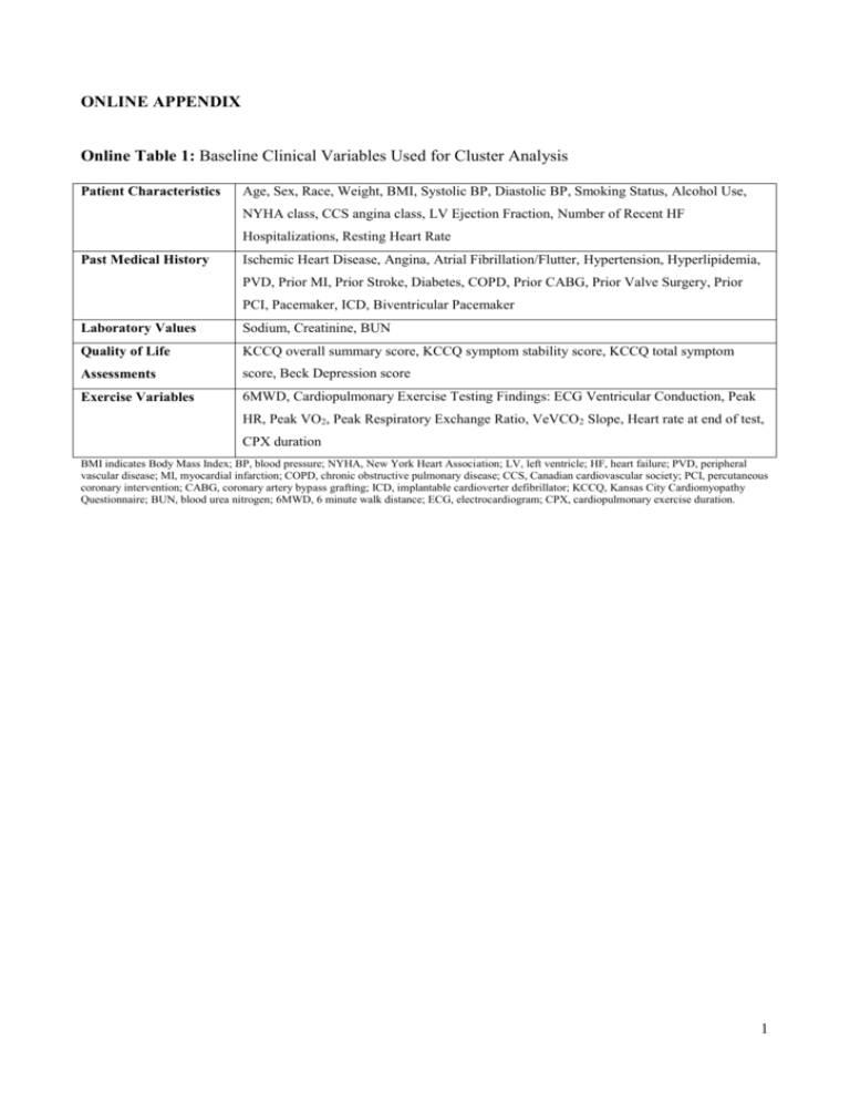
ONLINE APPENDIX
Online Table 1: Baseline Clinical Variables Used for Cluster Analysis
Patient Characteristics
Age, Sex, Race, Weight, BMI, Systolic BP, Diastolic BP, Smoking Status, Alcohol Use,
NYHA class, CCS angina class, LV Ejection Fraction, Number of Recent HF
Hospitalizations, Resting Heart Rate
Past Medical History
Ischemic Heart Disease, Angina, Atrial Fibrillation/Flutter, Hypertension, Hyperlipidemia,
PVD, Prior MI, Prior Stroke, Diabetes, COPD, Prior CABG, Prior Valve Surgery, Prior
PCI, Pacemaker, ICD, Biventricular Pacemaker
Laboratory Values
Sodium, Creatinine, BUN
Quality of Life
KCCQ overall summary score, KCCQ symptom stability score, KCCQ total symptom
Assessments
score, Beck Depression score
Exercise Variables
6MWD, Cardiopulmonary Exercise Testing Findings: ECG Ventricular Conduction, Peak
HR, Peak VO2, Peak Respiratory Exchange Ratio, VeVCO2 Slope, Heart rate at end of test,
CPX duration
BMI indicates Body Mass Index; BP, blood pressure; NYHA, New York Heart Association; LV, left ventricle; HF, heart failure; PVD, peripheral
vascular disease; MI, myocardial infarction; COPD, chronic obstructive pulmonary disease; CCS, Canadian cardiovascular society; PCI, percutaneous
coronary intervention; CABG, coronary artery bypass grafting; ICD, implantable cardioverter defibrillator; KCCQ, Kansas City Cardiomyopathy
Questionnaire; BUN, blood urea nitrogen; 6MWD, 6 minute walk distance; ECG, electrocardiogram; CPX, cardiopulmonary exercise duration.
1
Online Table 2. Baseline Characteristics of HF-ACTION Patients According to Inclusion in
Cluster Analysis
Characteristic
Total (N=2331)
Included
(N=1619)
Excluded (N=712)
P
59 (51-68)
59 (51-68)
60 (51-68)
012
28
27
31
0.11
Black, %
33
34
29
White, %
62
61
65
Other, %
5
5
6
30 (26-35)
30 (26-35)
30 (26-35)
0.51
Systolic BP, mmHg
111 (100-126)
112 (100-126)
110 (100-126)
0.42
Diastolic BP, mmHg
70 (60-78)
70 (62-80)
70 (60-78)
0.44
Heart Rate at Rest, bpm
70 (63-77)
70 (63-76)
70 (63-79)
0.12
Never
37
38
36
Current
17
16
19
Past
46
46
45
43
44
41
Age, years
Female Sex, %
Race
2
BMI, kg/m
0.06
Smoking Status
Alcohol Use
0.16
Patient Status
0.23
HF Hospitalizations prior 6
months
0.95
None, %
74
73
74
1, %
20
20
19
2, %
4
4
4
≥ 3, %
2
2
2
51
51
52
0.90
25 (20-30)
25 (20-30)
25 (20-30)
0.47
Ischemic Etiology, %
LVEF, %
NYHA Class
0.006
NYHA II, %
63
66
59
NYHA III, %
36
34
40
NYHA IV, %
1
1
1
Hypertension
60
62
56
0.01
Diabetes
32
33
31
0.36
Atrial Fibrillation or Flutter
21
21
21
0.92
Hyperlipidemia
66
66
65
0.61
Myocardial Infarction
42
42
42
0.78
Stroke
10
11
10
0.48
PVD
7
7
7
0.94
COPD
11
11
11
0.93
Prior Valve Surgery
6
5
6
0.61
Prior PCI
23
23
24
0.38
Patient History
2
Prior CABG
26
26
24
0.15
139 (137-141)
139 (137-141)
139 (137-141)
0.53
Potassium, mmol/L
3.7 (0.0-4.3)
3.7 (0.0-4.4)
3.6 (0.0-4.3)
0.73
Glucose, mmol/L
5.8 (5.1-7.2)
5.7 (5.1-7.2)
5.9 (5.1-7.4)
0.19
Creatinine, mg/dL
1.2 (1.0-1.5)
1.2 (1.0-1.5)
1.2 (1.0-1.5)
0.60
20 (15-28)
20 (15-27)
22 (16-30)
0.01
ACE-I or ARB
94
94
95
0.62
Beta Blocker
95
95
94
0.12
Loop Diuretic
78
79
76
0.08
Digoxin
45
47
40
<0.001
Implantable Cardioverter
Defibrillator
40
42
37
0.05
Biventricular Pacemaker
18
19
17
0.24
Pacemaker
18
17
19
0.51
14.4 (11.5-17.7)
14.5 (11.7-17.7)
14.2 (11.1-17.7)
0.03
33 (28-39)
32 (28-38)
33 (28-39)
0.07
371 (299-435)
375 (305-438)
359 (274-428)
<0.001
KCCQ Overall Summary
Score
68 (51-83)
69 (52-83)
67 (50-82)
0.09
Beck Depression Score
8 (4-15)
8 (5-15)
8 (4-15)
0.70
NT-proBNP, pg/mL
815 (341-1805)
796 (337-1854)
844 (351-1742)
0.61
Galectin-3, ng/mL
14.0 (11.0-18.6)
14.1 (11.0-18.7)
13.7 (11.0-18.4)
0.61
ST2, ng/mL
23.7 (18.6-31.8)
23.8 (18.4-31.7)
23.7 (18.8-32.3)
0.47
Patient Labs
Sodium, mmol/L
Blood Urea Nitrogen, mg/dL
Patient Meds
Patient Implant/Rhythm
Patient Exercise
Peak Oxygen Consumption,
mL/kg/min
VeVCO2 Slope
6 Minute Walk Distance, m
Patient Quality of Life
Patient Biomarkers
BMI indicates Body Mass Index; BP, blood pressure; NYHA, New York Heart Association; LVEF, left ventricle ejection fraction;
HF, heart failure; PVD, peripheral vascular disease; COPD, chronic obstructive pulmonary disease; CCS, Canadian Cardiovascular
Society; PCI, percutaneous coronary intervention; CABG, coronary artery bypass grafting; ACE-I, angiotensin converting enzyme
inhibitor; ARB, angiotensin receptor blocker; NT-proBNP, amino terminal proB-type natriuretic peptide.
3
Statistical Methods
The primary focus of this study was to identify clusters patients with different chronic systolic HF
phenotypes. The process is outlined as follows.
Variable Dimension Reduction
Forty-five baseline variables representing patient characteristics, medical history, labs, quality of
life scores, and exercise capabilities were identified for this aim. Given this large set of variables,
we sought to reduce the dimension of our covariate list through variable clustering. A procedure
(SAS PROC VARCLUS) was run separately for continuous and binary variables resulting in 6
clusters of continuous variables and 7 clusters of categorical variables. In brief, the SAS procedure
PROC VARCLUS is an iterative process that divides a large set of variables into several disjoint
clusters. At each iteration the procedure takes a given set of variables, identifies the first two
principal components of those variables, and assigns each variable to the component with which it
has strongest correlation. As a result, variables are aggregated into several non-overlapping
clusters. For each variable cluster, a summary score, as a linear combination of variables within the
cluster, can be derived for each patient. The coefficients of the variable cluster summary score are
identified by the first principal component of the variable cluster.
Variable clustering was done separately for continuous and categorical variables. The
underlying theory of principal components includes an assumption of multivariate normality.
However, this assumption is relaxed when principal components are used as a descriptive technique
(1). Here, we make no inference on the identified principal components and instead, only use them
to categorize variables. Furthermore, for data in which all variables are binary, PCA does provide a
plausible low-dimensional representation (2). Thus, we opt to separately analyze continuous
variables and binary variables in an attempt to best identify a lower-dimension of variables that
adequately describe the data.
Stopping rules for determining the appropriate number of continuous and categorical
clusters were as follows. At each stage, a cluster is broken and variables reassigned. We evaluate (a)
4
total proportion of variation in the variables explained by the variable clusters, (b) the second
eigenvalue of each cluster, (c) the change in the proportion of variation explained by the new
clustering compared to the prior iteration, (d) the change in the highest second eigenvalue from one
iteration to the next, and (e) potentially using clinical input to see if the clustered variables make
intuitive sense (blinded to the consequences on later steps in the process). For example, increasing
the number of continuous variable clusters up to 4 yielded a relative increase in variation explained
>10% compared to each prior iteration, whereas more than 4 continuous variable clusters yielded
less increase.
Patient Clustering
Given 13 scores for each patient after the variable reduction process, we next sought to identify
clusters of similar patients. We standardized the 13 scores to have mean zero and a standard
deviation of 1. After standardizing scores, using Ward’s minimum variance method of clustering
(implemented with SAS procedure PROC CLUSTER) we identified 4 patient clusters (3,4).
In brief, this is an agglomerative hierarchical clustering approach where we start with each patient
as his/her own singleton cluster and we iteratively merge clusters together. When two clusters have
been merged, they remain so for the remainder of the algorithm process.
For Ward’s minimum variance method, at each stage we define the distance between two clusters K
and L as
𝐷𝐾,𝐿
∑𝑗(𝑥𝐾,𝑗 − 𝑥𝐿,𝑗 )
=
1
1
𝑛𝐾 + 𝑛𝐿
2
where j indexes the cluster’s 13 variable scores. That is, 𝑥𝐾,𝑗 is the value of the jth standardized
variable score for cluster K and 𝑛𝐾 is the number of original patients in cluster K at that stage. Put
another way, at any stage the distance between two clusters is defined as a function of the sum of
squared differences in standardized scores. The distance is calculated between every possible
combination of two clusters.
5
The two clusters with the smallest distance are merged and new scores (say, merging K and
L forms a new cluster called M) 𝑥𝑀,𝑗 are an average of scores from patients in the new cluster.
Given N total patients in the sample, the process is iterative for N-1 steps until all patients have
been merged into a single
cluster. Ties in distance at any
stage are broken arbitrarily,
but in practice ties only occur
at early stages. At each
iteration, a cubic-clustering
criterion, pseudo F statistic,
and pseudo t2 statistic are
calculated (4). We also
calculate the semi-partial R2 at
Figure 1
each iteration which roughly measures loss of homogeneity within clusters caused by their merger.
Thus, small values of the semi-partial R2 indicate that two similar clusters have been merged
whereas large values indicate the merger of two heterogeneous clusters. A dendrogram (tree
diagram) is provided according to the semi-partial R2 describing the clustering process in this
analysis. The decision to use 4 patient clusters was based on an a priori criteria of at least 200
patients per cluster to promote stability of effect estimates, but blinded to outcomes and response to
exercise therapy. To assess the stability of the identified clusters, we used a bootstrap resampling
method and applied the original clustering algorithm to create various numbers of clusters (K=2,3…
10) in 1000 permutated datasets. We then compared the bootstrap clustering to the original data
clustering using the BK statistic, as proposed in Fowlkes and Mallows “A method for comparing
two hierarchical clustering”, to assess whether our clusters were more similar than what would be
expected with random allocation alone (7). The BK statistic is a representation of the similarity
6
between clusters, with a higher value indicating greater similarity. The overall BK estimate is the
average over the 1000 bootstrap samples and decreases with increasing number of clusters. The
observed BK from the bootstrap samples for all K was significantly larger than the expected value
had there been no correlation between each bootstrap clustering and the original clustering, and, as
expected, we observed a decrease in average BK across K=2,3….10. We found that the observed BK
was significantly larger than the expected BK in 999 of the 1000 bootstrap samples. Furthermore,
we observed a relatively large decrease in BK when moving from 4 to 5 clusters, indicating that
there is a substantial gain in similarity when using the threshold of 4 clusters (Figure). Therefore,
the BK statistic indicates that our clustering method is better than random allocation for all K and
supports the use of 4 clusters for this analysis.
Figure 2:
Evaluation
Baseline patient characteristics, labs, and medications are described according to the 4 identified
clusters. Continuous variables are described as median and 25th - 75th percentiles; categorical
7
variables are described as percentage. Characteristics are compared across clusters using a KruskalWallis test for continuous variables and Pearson chi-square test for categorical variables.
Outcomes and Response to Exercise Therapy
As an exploratory illustration, we assessed the association between cluster membership and clinical
outcomes using Cox proportional hazards regression. The primary endpoint was the composite allcause mortality or hospitalization. Secondary endpoints included all-cause mortality,
cardiovascular (CV) mortality or CV hospitalization, and CV mortality or HF hospitalization.
Proportional hazards assumptions were assessed for cluster; no significant violations were detected.
Kaplan-Meier estimated mortality and rehospitalization rates were plotted.
Using interaction terms in a Cox regression model, we also assessed whether cluster
membership is associated with a differential response to randomized exercise therapy for each of
these outcomes. Finally, we assessed the interaction between treatment and cluster with the
endpoint of change in Peak VO2 from baseline to 3 months. Among patients in this analysis known
to be alive at 3 months, approximately 15.2% were missing a 3 month measurement. Prior
exploratory analyses suggested this missingness could be related to various patient characteristics
such that some patient subgroups are more likely to return for follow up than others. To account for
this potential bias, we assessed the relationship between cluster membership and change in Peak
VO2 using linear regression with inverse probability weighting. First, logistic regression assessed
the each individual’s probability of missing a 3 month value conditional on a large set of baseline
patient variables. Then, in the linear model for change in peak VO2, patients with an observation
were weighted by the inverse of their probability to be observed. In this way, some patients are
given more weight than others if they are likely to represent not just themselves but also other
individuals who were similar but did not have follow up recorded. The linear regression
assumption of homoscedasticity was assessed and change in peak VO2 was assessed for normality;
no violations were suggested.
8
Results are reported for clinical outcomes as hazard ratios (HR) and 95% confidence
intervals (CI) for each cluster in comparison to a reference cluster and an overall p-value is
provided to assess the relationship between cluster and outcome. In models with interactions, an
interaction p-value is provided. We also provide the estimated HR and 95%CI for exercise therapy
versus usual care within cluster subgroups. Finally, results for change in peak VO2 are reported for
the interaction p-value. The estimated exercise therapy effect (and 95%CI) is presented for cluster
subgroups. For all analyses, P<0.05 was considered significant.
References:
1. Jolliffe, I. Principal component analysis. John Wiley & Sons, Ltd. 2005.
2. Gower, JC. Some distance properties of latent root and vector methods used in multivariate
analysis. Biometrika, 1966. 53(3-4), 325-338.
3. Sarle, WS. Cubic Clustering Criterion, SAS Technical Report A-108, Cary, NC: SAS
Institute Inc. 1983.
4. Ward, JH, “Hierarchical Grouping to Optimize an Objective Function,” Journal of the
American Statistical Association, 58, 236–244. 1963.
5. Fowlkes EB, Mallows CL. A Method for Comparing Two Hierarchical Clusterings. Journal
of the American Statistical Association. 1983. Vol. 78, No. 383, 553-569
9