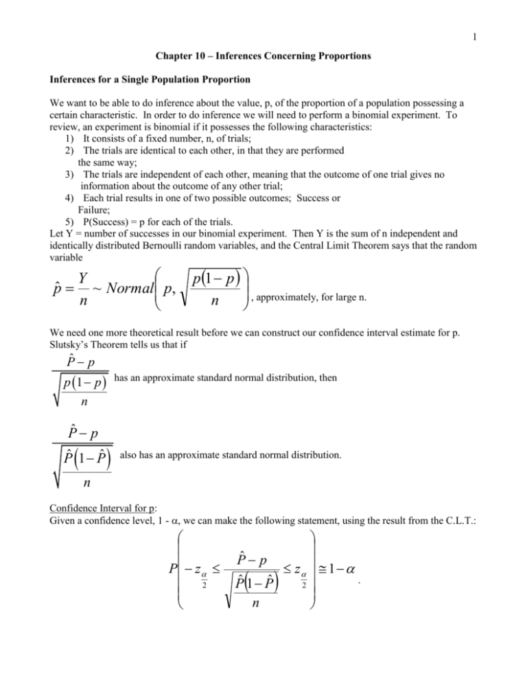
1
Chapter 10 – Inferences Concerning Proportions
Inferences for a Single Population Proportion
We want to be able to do inference about the value, p, of the proportion of a population possessing a
certain characteristic. In order to do inference we will need to perform a binomial experiment. To
review, an experiment is binomial if it possesses the following characteristics:
1) It consists of a fixed number, n, of trials;
2) The trials are identical to each other, in that they are performed
the same way;
3) The trials are independent of each other, meaning that the outcome of one trial gives no
information about the outcome of any other trial;
4) Each trial results in one of two possible outcomes; Success or
Failure;
5) P(Success) = p for each of the trials.
Let Y = number of successes in our binomial experiment. Then Y is the sum of n independent and
identically distributed Bernoulli random variables, and the Central Limit Theorem says that the random
variable
pˆ 

Y
~ Normal p,
n

p1  p  

 , approximately, for large n.
n

We need one more theoretical result before we can construct our confidence interval estimate for p.
Slutsky’s Theorem tells us that if
Pˆ  p
p 1  p 
n
Pˆ  p

Pˆ 1  Pˆ

has an approximate standard normal distribution, then
also has an approximate standard normal distribution.
n
Confidence Interval for p:
Given a confidence level, 1 - , we can make the following statement, using the result from the C.L.T.:



P  z  
 2




Pˆ  p

 z   1  
.
Pˆ 1  Pˆ
2 

n



2
Rearranging, we obtain:




Pˆ 1  Pˆ
Pˆ 1  Pˆ

ˆ
ˆ
P P  z
 p  P  z

n
n
2
2

Hence an approximate (1 - )100% confidence interval estimate for p is
   1  


Pˆ  z 
2
.

Pˆ 1  Pˆ
n

.
Example: p. 282, Exercise 10.3
Sample Size for a Specified Margin of Error:
As part of our experimental design, we want to specify the margin of error, E, that is acceptable for our
estimate of p, and choose a sample size to insure that we achieve this margin of error. We let
E  z
2
p 1  p 
n
. Solving for n, we obtain
 z
n 2
 E


2

 p 1 p
.
 


Now, we know E and , but we need to find a usable value for
p(1-p) before we can find the sample size. We use the fact that for any value of p between 0 and 1, we
have p(1-p)  0.25. Then
 z
n 2
 E


2

 1
 4


gives us an upper bound on the sample size that will insure that we will achieve our
desired margin of error with confidence level 1 - .
Example: p. 283, Exercise 10.11
Testing Hypotheses Concerning a Proportion:
We want to test hypotheses of the following possible forms:
1) H0: p = p0 vs. Ha: p  p0
2) H0: p  p0 vs. Ha: p < p0
3) H0: p  p0 vs. Ha: p > p0
The test statistic to be used is
Z
Pˆ  p0
p0 1  p0 
n
. Under the null hypothesis, the Central Limit
Theorem says that this statistic has an approximate standard normal distribution.
3
For the three types of alternative hypotheses, the rejection regions are:
1) Ha: p  p0
Reject H0 if |z| > z(/2)
2) Ha: p < p0
Reject H0 if z < -z()
3) Ha: p > p0
Reject H0 if z > z()
Example: p. 290, Exercise 10.19
Inference for Two Population Proportions Using Independent Samples
We have two separate populations and one specified characteristic. We want to compare the
proportion of members of population 1 who have this characteristic to the proportion of members of
population 2 who have the characteristic.
For population 1: p1 = proportion of population 1 who have the characteristic of interest, n1 = size of
random sample selected from population 1, and
characteristic.
p̂1 = proportion of sample 1 who have the
For population 2: p2 = proportion of population 2 who have the characteristic of interest, n2 = size of
random sample selected from population 2, and
characteristic.
p̂ 2 = proportion of sample 2 who have
We want to test one of the following alternative hypotheses against the appropriate null hypothesis.
Ha: p1 – p2  0
Ha: p1 – p2 > 0
Ha: p1 – p2 < 0
The parameter of interest to us is p1 – p2, and its point estimator is
pˆ 1  pˆ 2
. If both samples are
pˆ  pˆ
large, then the sampling distribution of
1
2 is approximately normal, and the following
random variable has an approximate standard normal distribution:
Z
 pˆ 1  pˆ 2    p1  p 2 
p1 1  p1  p 2 1  p 2  .

n1
n2
To test any of the above alternative hypotheses against the corresponding null hypothesis, we use the
following statistic:
4
Z
 pˆ 1  pˆ 2 
1
1 
p (1  p )  
 n1 n2 
, where
p
n1 pˆ 1  n2 pˆ 2
n1  n2
is the average of the two
sample proportions. Under the null hypothesis, this statistic has an approximate standard normal
distribution.
Example: Photolithography plays a central role in manufacturing integrated circuits made on thin discs
of silicon. Prior to a quality-improvement program, too many rework operations were required. In a
sample of 200 units, 26 required reworking of the photolithographic step. Following training in the use
of Pareto charts and other approaches to identify significant problems, a new sample of size 200 had
only 12 that needed rework. Is this sufficient evidence to conclude at the 0.01 level of significance that
the improvements have been effective in reducing the rework?
Confidence Interval for a Difference of Population Proportions
We want to estimate the difference between the proportion of population 1 who have a characteristic of
interest and the proportion of population 2 who have the characteristic. The formula for the (1 –
)100% confidence interval is
 pˆ 1  pˆ 2   z 
2
pˆ 1 1  pˆ 1  pˆ 2 1  pˆ 2 

.
n1
n2
Example: In the previous example, we want an approximate 99% confidence interval estimate of the
difference between the proportion of units requiring rework after the improvement program and the
proportion of units requiring rework prior to the improvement program.