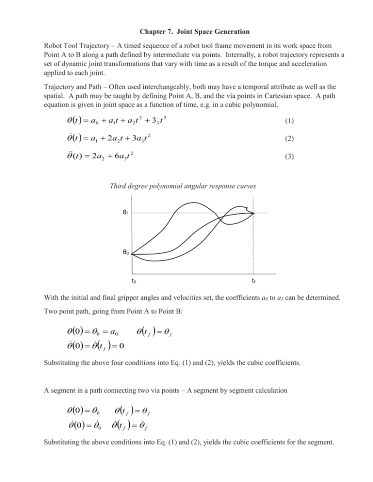
Chapter 7. Joint Space Generation
Robot Tool Trajectory – A timed sequence of a robot tool frame movement in its work space from
Point A to B along a path defined by intermediate via points. Internally, a robot trajectory represents a
set of dynamic joint transformations that vary with time as a result of the torque and acceleration
applied to each joint.
Trajectory and Path – Often used interchangeably, both may have a temporal attribute as well as the
spatial. A path may be taught by defining Point A, B, and the via points in Cartesian space. A path
equation is given in joint space as a function of time, e.g. in a cubic polynomial,
 t   a0  a1t  a2 t 2  33 t 3
(1)
t   a1  2a2 t  3a3t 2
(2)
(t )  2a2  6a3t 2
(3)
Third degree polynomial angular response curves
θf
θ0
t0
tf
With the initial and final gripper angles and velocities set, the coefficients a0 to a3 can be determined.
Two point path, going from Point A to Point B:
 0   0  a0
0  t f   0
 t f    f
Substituting the above four conditions into Eq. (1) and (2), yields the cubic coefficients.
A segment in a path connecting two via points – A segment by segment calculation
 0   0
0   0
 t f    f
t f    f
Substituting the above conditions into Eq. (1) and (2), yields the cubic coefficients for the segment.
Parabolic path with linear acceleration
Velocity
Angular Position
Acceleration
Linear path with parabolic blends
Angular Position
Acceleration
Velocity
θ"
θ"t1
0
0
t2
t12
t1
-θ"
0
t2
Interpolation - Movement between via points. Linear (straight line) or Polynomial (curved).
All robot joints, including the prismatic joints, are motor driven. Therefore, intuitively a linear motion
with a high degree of accuracy is more difficult to achieve than a non-linear motion.
The robot arm normally pass near, not through, the via points to avoid jerky motion unless instructed
to do so. If no via points are specified, the robot will take a smooth “PTP” path.
Homework #9
Solve (6.8) – Forward velocities and accelerations only.
Solve (7.2), (7.5), (7.7), (7.10), Due 11/25. Study Examples and (7.17).
Path Generation – Liner Path with parabolic blends
The path will bypass the via points in blending process without touching them.
θt
θ2
θ4
t 23 ,23
t12 , 12
t3, θ3
θ1
t1
t12
T12
t2
T23
Linear Path with Parabolic Blends
t
Design attributes – Segment duration (linear and blend), velocity of the linear segment, acceleration
of the blend,
For interior points
23  ( 3   2 ) / T23
t 3  (34  23 ) / 3
t 23  T23 
1
1
t 2  t3
2
2
where T23=t2+t23+t3
For end points, starting with the relationship to find the blending time t1
1t1  ( 2  1 ) /(T12 
1
t1 )
2
2
t1  T12  T12  2( 2  1 ) / 1
12  ( 2  1 ) /(T12 
t12  T12  t1 
1
t1 )
2
1
t2
2
Pseudo via points – when the path must go through the via points.
θt
t
Linear Path with Parabolic Blends over
Pseudo via points for through points