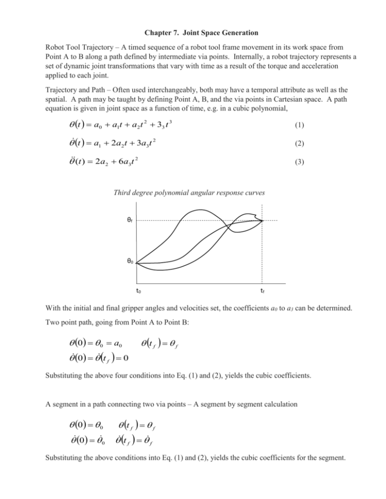
Chapter 7. Joint Space Generation
Robot Tool Trajectory – A timed sequence of a robot tool frame movement in its work space from
Point A to B along a path defined by intermediate via points. Internally, a robot trajectory represents a
set of dynamic joint transformations that vary with time as a result of the torque and acceleration
applied to each joint.
Trajectory and Path – Often used interchangeably, both may have a temporal attribute as well as the
spatial. A path may be taught by defining Point A, B, and the via points in Cartesian space. A path
equation is given in joint space as a function of time, e.g. in a cubic polynomial,
 t   a0  a1t  a2 t 2  33 t 3
(1)
t   a1  2a2 t  3a3t 2
(2)
(t )  2a2  6a3t 2
(3)
Third degree polynomial angular response curves
θf
θ0
t0
tf
With the initial and final gripper angles and velocities set, the coefficients a0 to a3 can be determined.
Two point path, going from Point A to Point B:
 0   0  a0
0  t f   0
 t f    f
Substituting the above four conditions into Eq. (1) and (2), yields the cubic coefficients.
A segment in a path connecting two via points – A segment by segment calculation
 0   0
0   0
 t f    f
t f    f
Substituting the above conditions into Eq. (1) and (2), yields the cubic coefficients for the segment.
Angular Position
Velocity
Angular Position
Velocity
Acceleration
Acceleration
0
0
0
Interpolation - Movement between via points. Linear (straight line) or Polynomial (curved).
All robot joints, including the prismatic joints, are motor driven. Therefore, intuitively a linear motion
with a high degree of accuracy is more difficult to achieve than a non-linear motion.
The robot arm normally pass near, not through, the via points to avoid jerky motion unless instructed
to do so. If no via points are specified, the robot will take a smooth “PTP” path.
θ
t2, θ2
θ4
t12 , 12
θ3
t1, θ1
T12
t
Linear Path with Parabolic Blends
Design attributes – Segment duration (linear and blend), velocity of the linear segment, acceleration
of the blend,
For interior points
23  ( 3   2 ) / T23
t 3  (34  23 ) / 3
t 23  T23 
1
1
t 2  t3
2
2
where T23=t2+t23+t3
For end points
1t1  ( 2  1 ) /(T12 
1
t1 )
2
Solving for t1.
t1  T12  T12  2( 2  1 ) / 1
2
12  ( 2  1 ) /(T12 
t12  T12  t1 
1
t1 )
2
1
t2
2
θ
t
Linear Path with Parabolic Blends over
Pseudo via points for through points
Linear Positioning System
Control Resolution Distance between two adjacent addressable points.
Set by desired control needs and constrained by mechanical limits.
Addressable Points Set by the step angle, the gear/pulley ratio, and the lead screw pitch.
Accuracy (Maximum error)
½ of Control Resolution + 3σ (Standard Deviation of positional variability)
Repeatability (Precision)
±3σ
Control
Resolution
Accuracy
Max. error
Precision
±3σ
Work Table
TaTable
Servo
Motor
Reduction
Lead Screw
Recirculating Ball
Gear
Bearing Nut
Pulse Output
Encoder
Pitch
Stepper
Motor
Lead Screw Nut assemblies
Encoder Disk
Pulse (Baud) Rate = Motor RPM x 360 / Step Angle