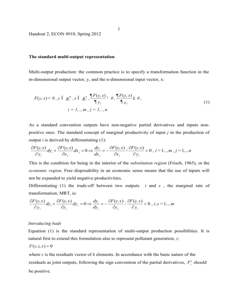
1
Handout 2, ECON 4910, Spring 2012
The standard multi-output representation
Multi-output production: the common practice is to specify a transformation function in the
m-dimensional output vector, y, and the n-dimensional input vector, x:
F ( y, x) = 0 , y Î R+m , x Î R+n ,
¶ F ( y, x)
¶ F ( y, x )
³ 0,
£ 0,
¶ yi
¶ xj
(1)
i = 1,..,m , j = 1,..,n
As a standard convention outputs have non-negative partial derivatives and inputs nonpositive ones. The standard concept of marginal productivity of input j in the production of
output i is derived by differentiating (1):
F (y,x)
F (y,x)
dy
F (y,x ) F (y,x )
dyi 
dx j  0  i  
/
 0 , i = 1,..,m , j = 1,..,n
 yi
x j
dx j
x j
 yi
This is the condition for being in the interior of the substitution region (Frisch, 1965), or the
economic region. Free disposability in an economic sense means that the use of inputs will
not be expanded to yield negative productivities.
Differentiating (1) the trade-off between two outputs
i and s , the marginal rate of
transformation, MRT, is:
F (y,x )
F (y,x )
dy
F (y,x ) F (y,x )
dyi 
dys  0  i  
/
 0 , i, s = 1,..,m
 yi
ys
dys
ys
 yi
Introducing bads
Equation (1) is the standard representation of multi-output production possibilities. It is
natural first to extend this formulation also to represent pollutant generation, z:
F (y,z,x )  0
where z is the residuals vector of k elements. In accordance with the basic nature of the
residuals as joint outputs, following the sign convention of the partial derivatives, Fz should
be positive.
2
Introducing a social planning problem
Evaluating pollutants through the monetised damage function
D  D (z1 ,.., zk ) ,
D
 0, s  1,..., k
zs
Introducing a demand funtion (on price form) for each good the social planning problem for a
single (representative) firm, characterised by some multiple-output technology
m
yi

Max
i 1 wi 0
n
pi ( wi )dwi   q j x j  D( z1 ,..., zk )
j 1
subject to
a multiple output technology
Pollutants as outputs in the standard formulation
The Lagrangian function is:
m
L
yi

i 1 wi 0
n
pi ( wi )dwi   q j x j  D( z1 ,..., zk )   F ( y , z, x )
j 1
The necessary first order conditions
L
 pi   Fyi  0 (  0for yi  0), i  1,.., m
yi
L
  q j   Fxj  0(  0for x j  0), j  1,.., n
x j
L
  Dzs   Fzs  0 (  0for zs  0), s  1,.., k
zs
  0(  0 for F ( y , z, x )  0)
Interior solutions
pi
 Fxj
Fyi
 q j , i  1,.., m , j  1,.., n
From the last condition of the necessary conditions above it follows that the generation of the
polluting residual should be set to zero since equality cannot be optimal in the case
considered here. Since there is no explicit formalisation of the inevitability of residuals in the
formulation F (y,z,x )  0 when using inputs, this is the logical result, pollutants being bads
in the objective function. The maximal flexibility of the multiple-output modelling, implying
that inputs can be directed to the production of any of the outputs, leads inevitably to
intuitively nonsensical results that zero bads can be achieved at no costs; inputs are simply
3
reallocated without costs to produce more of goods with a positive value and to produce
zero of bads with negative values. Therefore, it does not have a good meaning to specify
residuals as joint outputs as in F (y,z,x )  0 . A single transformation function does not give
enough structure to allow bads to be cast as outputs.
Pollutants as inputs
Since the sign of Fzs now is negative in the last necessary condition in (10), the condition is
formally identical to the condition for employing an input, leading to a positive level of
pollutants generation in the case of an interior solution. The factor price is replaced with the
marginal damage. There are, however, several weaknesses with this formulation. When the
multi output technology has a maximal degree of assortment with bads formally as inputs,
i.e., Fzs  0 , we have:
i) the socially optimal level of bads is only determined as a trade-off with goods,
ii) no explicit purification activity in the form of inputs can be identified.
Generation of pollutants acts as any other input, and thus has a positive impact on every
output in general. The pollutants are thus associated with outputs, not with inputs. Using the
necessary conditions the trade-off between outputs and residuals generation is expressed by:
Dzs  pi
 Fzs
Fyi
 pi  Dzs
Fyi
 Fzs
, i  1,.., m , s  1,.., k
The first expression says that polluting residuals should be employed up to the point that the
value of the resulting output i is equal to the marginal damage caused by the pollutant. The
second, equivalent, expression shows that the marginal value of the output in question is
equal to the damage evaluation of the marginal unit requirement of pollutants generation.
There is thus a formal trade-off mechanism in place linking outputs and pollutants, so if this
is the connection we want to model at the micro level, we have at least a qualitative
representation, but not a correct quantitative one, since an active part of the resource base is
left outside the explicit modelling. Most awkwardly, purification activity is swept under the
carpet.
So if one is interested in optimal abatement per se this is not the appropriate
formulation.
Abatement by input substitution cannot be captured either because there is no link between
the “real” inputs, x, and the residuals generation, z, specified as input. The model
4
specification allows low sulphur coal to be substituted for high sulphur coal when factor
prices change, but this has no impact on generation of sulphur as a residual! There is a price
to be paid for violating the engineering principles of production. A problem is the substitution
between inputs and bads as inputs. If the bad is SO2 and the input is coal in the generation of
electricity, there is, of course, no substitution between these two variables.
The Frisch multi-output model
The case of freedom in directing inputs into any output is termed assorted production in
Frisch (1965). The core production function apparatus of Frisch (1965), Part four) is based on
these concepts, and may be described by a set of functions :
¶ Fi
¶ Fi
(
,..,
,
,..,
)
=
0
,
³
0
,
£ 0,
y
y
xn
F 1
m x1
¶ ys
¶ xj
i
i = 1,.., μ , s = 1,..,m , j = 1,..,n
The relation between number of outputs and equations is defined as the degree of assortment:
 = m - . A special case is  = 1. We are then back to the common textbook specification (1)
of multiple outputs. The degree of assortment is then m - 1, or in the Frisch spirit m-1 dimensional freedom of assortment, i.e. the maximal degree. The flexibility in combining
outputs and inputs is maximal. A negative number means that there exist one or more pure
factor bands, i.e. there are relationships as part of (2) between inputs independent of outputs,
Fb(x1,..,xn) = 0. In the case of specific technical relations between products Frisch talks about
couplings between the outputs. The product couplings restrict the freedom of combining
outputs. The degree of couplings, , is the number of relations between outputs, in the
system (2), independent of inputs, Fc(y1,..,ym) = 0. Note that the sign convention for partial
derivatives does not apply to factor bands or product couplings. Obviously the direction of a
coupling, e.g. dyc1 / dyc2 = -Fyc2c/ Fyc1c is unrestricted in sign, as well as the corresponding
direction within a factor band. Thus the sign convention applies to relations in (2) with both
outputs and inputs simultaneously present only.
A special case of (2) is the case of no assortment. We will later argue that this case is of
especial relevance for pollution modelling. Frisch calls this case factorially determined multioutput production. Introducing z as pollutants generated in the production of y:
i
y i = f ( x1,.., x n ) , i = 1,..,m
z  g ( x1,.., x n )
(3)
5
The degree of assortment is (m - m) = 0, meaning that for a given set of inputs, all the
outputs are determined. However, this is not the same as output couplings. There are output
isoquant maps for each function in (3). To the degree that these do not coincide, we will
realise outputs in different proportions varying the inputs. In the terminology of Frisch, we
have product separation. If the isoquant maps coincide completely we then have the case of
couplings, i.e. the outputs cannot be separated. The coupling may be proportional at the
simplest, or exhibiting more complex variability. (See Figure 1 for illustrations.)