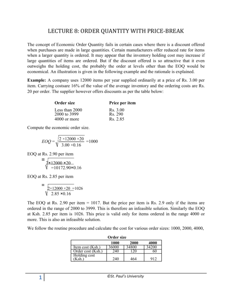
LECTURE 8: ORDER QUANTITY WITH PRICE-BREAK
The concept of Economic Order Quantity fails in certain cases where there is a discount offered
when purchases are made in large quantities. Certain manufacturers offer reduced rate for items
when a larger quantity is ordered. It may appear that the inventory holding cost may increase if
large quantities of items are ordered. But if the discount offered is so attractive that it even
outweighs the holding cost, the probably the order at levels other than the EOQ would be
economical. An illustration is given in the following example and the rationale is explained.
Example: A company uses 12000 items per year supplied ordinarily at a price of Rs. 3.00 per
item. Carrying costsare 16% of the value of the average inventory and the ordering costs are Rs.
20 per order. The supplier however offers discounts as per the table below:
Order size
Price per item
Less than 2000
2000 to 3999
4000 or more
Rs. 3.00
Rs. 290
Rs. 2.85
Compute the economic order size.
EOQ =
2 ×12000 ×20
=1000
3.00 ×0.16
EOQ at Rs. 2.90 per item
=
2×12000 ×20
=10172.90×0.16
EOQ at Rs. 2.85 per item
=
2×12000 ×20 =1026
2.85 ×0.16
The EOQ at Rs. 2.90 per item = 1017. But the price per item is Rs. 2.9 only if the items are
ordered in the range of 2000 to 3999. This is therefore an infeasible solution. Similarly the EOQ
at Ksh. 2.85 per item is 1026. This price is valid only for items ordered in the range 4000 or
more. This is also an infeasible solution.
We follow the routine procedure and calculate the cost for various order sizes: 1000, 2000, 4000,
Item cost (Ksh.)
Order cost (Ksh.)
Holding cost
(Ksh.)
1
Order size
1000
2000
36000
34800
240
120
240
464
©St. Paul’s University
4000
34200
60
912
Exercises
1. Assume the following price structure
Units
0-199
200-399
400-599
600
Units Price
Rs. 10.00
9.75
9.50
9.25
Purchase cost per order = Ks. 25
Cost of the item
= Ksh. 10
Annual demand
= 950 Units
Carrying cost
=Ksh2/Unit/yr
2. Find the optimal order quantity for a product for which the price-breaks are as follows:
Items q
0 ≤ q < 100
100 ≤ q < 200
200 ≤ q
Price/Unit
Rs. 20
Rs. 18
Rs. 16
The monthly demand for the product is 600 units. The storage cost is 15% of unit
cost and the cost of ordering is Ksh. 30 per order.
DYNAMIC ORDER QUANTITY
The basic assumption in the derivation of Economic Order Quantity models discussed
previously is that the demand is uniform. But in certain situations the demand is not uniform. It
may rise and fall, depending on seasonal influences. A general method is discussed below that
can be applied to any pattern of varying demand due to seasonal or irregular variations.
Consider the following example to illustrate how a varying demand problem can be
tackled. This is known as Dynamic Order Quantity model.
Example: The requirements for 12 months are given below:
Month
Requirement
Set up cost
Unit price
Interest
1
20
2
40
3
10
4
10
5
10
6
2
7
40
8
30
9
40
10
40
11
10
12
20
= Rs. 20
= Rs. 5 per item.
= 24% per
year
or 2% per month.
Solution: To calculate the dynamic order quantity we can adopt the following procedure.
The first month's requirement has to be ordered in the first month itself at a procurement cost of
Rs. 20. Now we have to decide whether the second month's requirement can also be ordered
along with first month's requirement. This involves additional carrying cost, but this will result in
saving an extra set up. Hence if the saving on set up costs outweighs the carrying costs, then we
2
©St. Paul’s University
include the second month's requirements along with the first month. Similarly a decision can be
taken whether to include the third month's requirement in the first month itself. This procedure is
followed until the procurement costs and carrying costs are balanced.
Let n represent the month, n = 1, 2, ..., 12. Let Rn be the requirement during nth month and Rn+1
be the requirement during (n + 1)th month. If the (n + 1)th month requirement namely Rn+1 is
absorbed in nth month itself,
the additional procurement cost is saved.
Hence the saving in procurement cost is (C2/n). But the additional carrying cost is C3 n
(Rn+1). If the additional carrying cost is less than the procurement cost, then the (n+1)th month
requirement is to be ordered also
with nth month.
Hence we have to check whether
nRn + 1 C3 < C2/n
n2Rn + 1 < C2/C3
If the answer to the above inequality is yes, then, the future month's requirements are included in
the first month itself. If the answer is 'no', then that requirement is to be ordered afresh and this is
treated as month n = 1. In this example C2/C3 = 20/0.01 = 200. All the eleven information can
be represented in the table as shown.
Month.
Requirement. Rn
1
2
3
4
5
6
Total
7
8
9
Total
10
11
12
Total
20
40
10
10
10
2
92
40
30
40
110
40
10
20
70
n
n2Rn+1.
1
2
3
4
5
6
40
40
90
160
50
1440
Is
n2Rn+1<200
Yes
Yes
Yes
Yes
Yes
No
1
2
3
30
160
360
Yes
Yes
No
include 10 in 7th month.
include 40 in 7th month.
set up again in month 10
1
2
10
80
Yes
Yes
include 10 in month 10
include 20 in month 10
Action.
include 40 in month 1
include 10 in month 1
include 10 in month 1
include 10 in month 1
include 2 in month 1
set up again in month 7
Hence we order three times a year in the first month, seventh month and tenth month, the batch
sizes being 92, 110 and 70 respectively.
Exercise: Compute the dyanamic EOQ is for the following requirements.
Month
Requirement.
3
1
50
2
100
3
10
4
170
5
150
6
180
7
1
©St. Paul’s University
8
260
9
100
10
80
11
150
12
200
ABC ANALYSIS
The ABC analysis is the analysis that attracts management on those items where the greatest
savings can be expected. This is a simple but powerful tool of statistical sampling in the area of
inventory control or materials management.
In this analysis, the items are classified or categorized into three classes, A, B and C by their
usage value. The usage value is defined as,
The ABC concept is based on Pareto's law that few high usage value items constitute a major
part of th capital invested in inventories whereas a large number of items having low usage value
constitute an insignificant part of the capital. It too much inventory is kept, the ABC analysis can
be performed on a sample. After obtaining the random sample the following steps are carried out
for the ABC analysis
STEP 1: Compute the annual usage value for every item in the sample by multiplying the annual
requirements bythe cost per unit.
STEP 2: Arrange the items in decending order of the usage value calculated above.
STEP 3: Make a cumulative total of the number of items and the usage value.
STEP 4: Convert the cumulative total of number of items and usage values into a percentage of
their grand totals.
STEP 5: Draw a graph connecting cumulative % items and cumulative % usage value. The
graph is dividedapproximately into three segments, where the curve sharply changes its shape.
This indicates the three segments A, B and C.
The class A items whose usage values are higher are to be carefully watched and are under the
strict and continued scrutiny of the senior inventory control staff. These items should be issued
only an indents sanctioned by the staff. The class C items on the other extreme can be placed on
the shop floor and the personnel can help themselves without placing a formal requisition. The
class B items fall in between A and C.
ABC concept conforms to the consideration implied in the EOQ model. 'A' items have
high inventory carrying costs and should therefore be placed with EOQ concept. The 'C' items
require very little capital and have therefore low inventory carrying costs. Hence, they can be
purchased in bigger lots. 'B' items are usually placed under statistical stock control.
Example: Perform ABC analysis on the following sample of 10 items from an inventory.
1
Items
Annual
Usage
300
(Unit)
Unit
Cost
10
(Rs.)
4
2
3
4
5
6
7
8
9
10
2700
30
1000
50
220
160
800
600
70
15
10
5
4
100
5
5
15
10
©St. Paul’s University
Solution:
STEP 1: Calculate usage value by multiplying annual usage of each item with its unit cost and
tabulate them andassign rank by giving rank to the largest usage value as in table below.
Items No.
1
2
3
4
5
6
7
8
9
10
Annual Usage
3000
40500
300
5000
200
22000
800
4000
9000
700
Ranking
6
1
9
4
10
2
7
5
3
8
STEP 2: Arrange items as per ranking and calculate cumulative usage and % cumulative value
as in the table below.
Rank
1
2
3
4
5
6
7
8
9
10
Item No. Annual usage
2
6
9
4
8
1
7
10
3
5
40500
22000
9000
5000
4000
3000
800
700
300
200
Cumulative % of cumulative Cumulative %
Annual usage Annual usage
of item
40500
47
10
62500
73
20
71500
84
30
76500
91
40
80500
94.2
50
83500
98
60
84300
98.6
70
85000
99.4
80
85300
99.8
90
85500
100
100
If you draw the figure, you will see that the curve changes at points (say) X and Y. The items
upto X is classified as class A items and between X and Y as class B and the rest as class C
items.
SOME DEFINITIONS
Lead-time: This is defined as the time interval between the placing of the orders and the actual
receipt of goods.
Lead-time Demand: This is the lead-time multiplied by demand rate. For example, if the leadtime is 3 weeks andthe demand is at the rate of 50 items per week, then the lead-time demand is
3 x 50 = 150 items.
The lead-time may not be constant. For one batch, a vendor may take 45 days and for the next
batch 50 days and so on. Lead-time itself is therefore a stochastic variable. This complicates the
problem of accumulating stock over the period encompassed by the lead-time. Lead-time may
also be forecast exponentially as is done with the demand.
5
©St. Paul’s University
Safety stock or Buffer stock: Lead-time demand is the stock level, which, on the average is
sufficient to satisfy thecustomer's orders as the stocks are being replenished. "On the average"
would mean that during this period of replenishment 50% of the customer's order can be filled
and the remaining 50% may either be refused or back ordered to be filled later. The reason for
this is obvious. Forecast is after all a point estimate only. If the demand is greater than the
forecasts, the customers would not be serviced. If the demand is less then the forecasts,
overstocking would occur. When these two variables, stock level and service to the customer, are
summed up over thousands of stock level and service to the customer, are becomes a major
problem for an organisation to find an acceptable compromise between the two. Sometimes the
management in an organisation would like to limit the disservice to the customer down to 5% or
10% at the cost of extra stocking. This extra stock in excess of the lead-time demand is called the
safety stock. Saftely stock may be expressed as percentages of the lead-time demand. It may be
computed in different ways.
Reorder level: This is defined as the level of the inventory at which the order is placed. It has
generally twocomponents (i) Lead time Demand and (ii) Safety Stock.
Reorder level (ROL) = Lead time demand (LTD) + Safety stock (SS).
Computation of Safety Stock:
As discussed earlier, if the demand exceeds the forecast, the result is bad service to the customer
and if the demand is less than the forecast figure, this results in overstocking. Thus there is a
forecast error. This error is assumed to be normally distributed, with zero mean. If the standard
deviation of the forecast error is calculated, then safety stock may be set with the desired
confidence level to result in not more the 5 or 10% shortages etc.
There is another measure of variation, popularly known as mean absolute deviation (MAD),
which can be computed far more easily. It can be routinely smoothed every period for obtaining
better estimates of the safety stock.
MAD is related to the standard deviation for a normal distribution as given by.
MAD =2 πSD.
Therefore,
SD = π2MAD
Now safety stock = Z (S.D)
=Zπ2MAD
=K MAD
whereK is called service factor
K=Zπ2
The safety stock is for just one period and has to be extended over the lead time. The necessary
6
©St. Paul’s University
formula has been derived by extensive simulation by statisticians and is given below.
MADLT = (0.659+ 0.341 LT) MAD
Safety stock over the lead-time
=K(0.659 +0.341LT)MAD
=Zπ2(0.659+0.34LT)MAD
Example: A company uses annually 50000 units of raw materials at a cost Rs. 1.2 per item.
Ordering cost of items isRs. 45 per order and item carrying cost is 15% per year of the average
inventory.
1.
2.
Find the economic quantity.
Suppose that the company follows the EOQ policy and it operates for 300
days a year, that the procurement time is 12 days and mum, minimum and
average inventories.
Solution:
D = Demand = 50000/year C1 = Rs. 1.2 per item
No. of days = 300/year
C2 = Rs. 45 per order
Lead time = 12 days
C3 = 15% of Rs. 1.2/item/year. = Rs. 0.18 per item per year. Safety stock = 500
(1)EOQ=
2C D
2
=
C3
2×45 ×50000
0.18
= 25000000
=5000
(2) Requirement per day = 50000/300
Lead time demand = 12 x 500/3 = 2000
Safety stock
= 500
= Lead time demand+ safety
Reorder level stock
7
©St. Paul’s University
= 2000 + 500 = 2500
Maximum inventory = E.O.Q + Safety stock
= 5000 + 500 = 5500
Minimum
inventory
Average
inventory
= Safety stock = 500
= (Max. Inv. + Min.
Inv.)/2
= (5500 + 500)/2 = 3000
Example A scrutiny of past records gives the following distributions for lead time and daily
demand during lead time.
Lead time distribution
Lead time (days)
Frequency
3
2
4
3
5
4
6
4
7
2
8
2
9
2
10
1
Demand distribution
Demand/day
(units)
Frequency
0
2
1
4
2
5
3
5
4
4
What should be the buffer stock?
Solution:
Computation of average or mean lead time.
=∑ (Frequency ×lead time) ∑
Frequency
=6+12
+20 24+ 14+6 18+
10+ + 20
=6 days
Average demand
=∑ (Frequency ×demand/day) ∑
frequency
=0+4
+10 15+ 16+10 +6
14+ + 25
=3
Average lead-time demand
= Average lead time x Average demand/day
= 6 x 3 = 18.
Maximum lead-time demand.
= Max. lead time x Max. demand/day
8
©St. Paul’s University
5
2
6
1
7
2
= 10 x 7 = 70
∴ Buffer stock = Max. lead time demand - Average lead time demand
*Example 7.7.3
For a fixed order quantity system find the EOQ, SS, ROL and average inventory
for an item with the following data.
Demand = 10000
item unit cost= Re 1
Order cost = Rs.12
Holding cost = 24%
Post lead times = 13 days
Solution:
(1)
EOQ=
2C D
2
C
3
2×12 10000×
=
=1000 items
0.24×1
(2)
The Average lead time = (13 + 14 + 15 + 16 + 17)/5
= 15 days ( 30days time is omitted)
Maximum lead time = 30 days
Safety stock = ( 30 - 15) x 10000/(30 x 12) = 420
(3)
Reorder level = Lead time demand + Safety stock
= 417 + 420 = 837
(4)
Average inventory = (1420 + 420)/2
= 1840/2 = 920.
Example: An airline has determined that 10 spare brake cylinders will give them stock out
risk of 30%, whereas 14will reduce the risk to 15% and 16 to 10%. It takes 3 months to
receive items from supplier and the airline has an average of 4 cylinders per month. At what
stock level should they reorder assuming that they wish to maintain an 85% service level.
Solution:
Lead time demand = 3 x 4 = 12 items
9
©St. Paul’s University
Safety stock at 85% service
= 15% disservice
or 15% stock out risk
= 14 items
Reorder level = 12 + 14 = 26 items.
Example: Data on the distribution of lead time for a motor component were collected as
shown. Management wouldlike to set safety stock levels that will limit the stock out to 10%.
Lead time (weeks)
Frequency of
occurrence
1
2
3
4
5
6
7
8
10
20
70
40
30
10
10
10
How many weeks of safety stock are required to provide the desired service level?
Solution:
Lead time (weeks)
Frequency
1
2
3
4
5
6
7
8
10
20
70
40
30
10
10
10
200
Probability Cumulative
Probability
0.05
0.05
0.10
0.15
0.35
0.50
0.20
0.70
0.15
0.85
0.05
0.90
0.05
0.95
0.05
1.00
Average lead time = ∑(lead time x frequency)/ ∑frequency
= (10 + 40 + 210 + 160 + 150 + 60 + 70 + 80)/200
= 770/200 = 3.85 weeks
Upto 90% service level max.lead time is 6 weeks.
Hence 6 - 3.85 = 2.15 weeks of stock would provide the service level of 90%
(Note: If the lead time is given as a continuous time distribution take the mid point.)
Example: Demand for a product during an order period is assumed to be normally
distributed with mean of 1000units and standard deviation of 40 units. What % service can a
company expect to provide (i) if it satisfies the average demand only (ii) if it carries a safety
stock of 60 units.
Solution:
1.
10
If the company provides only average demand, we can expect only 50% service
©St. Paul’s University
2.
level.
The standard normal variate Z is computed with the following formula.
Z = (Safety stock - 0)/ Standard deviation
= (60 - 0)/40 =
1.5 The area under normal curve for Z =1.5
is 0.4332.
∴ Service level = 0.50 + 0.4332 = 0.9332 04 93.32%
Example: A manufacturer of water filters purchases components in EOQ's of 850 units/order.
Total demandaverages 12000 components per year and MAD = 32 units per month. If the
manufacturer carries a safety stock of 80 units, what service level does the this give the firm?
Solution:
Standard deviation =
2
×MAD =MAD / 0.8 32= / 0.8 40=
π
Z = (S S - 0)/S.D = (80 - 0)/40 = 2
The area under normal curve for Z = 2 = 0.4772.
Service level = 0.9772 or 97.72%
Example: A firm has normally distributed forecast of usage with MAD = 60 units. It desires
a service level, whichlimits the stock, outs to one order cycle per year.
(1) How much safety stock should be carried if the order quantity is normally a week's
supply?
(2) How much safety stock should be carried if the order quantity is weeks supply.
Solution:
No. of orders = 52/year.
1 stock out in 52 weeks means a 98 % = (51/52) values
For 98% area, the value of
Z = 2.05 (from tables)
S D = MAD/0.8 = 60/08
Z = (S S - 0 )/S D= (S S - 0)/60/0.8
2.05 = (S S - 0 ) x 0.8/60
SS = 2.05 x 60/0.8 = 154 units.
(a)Number of orders = 52/5
11
©St. Paul’s University
1 stock out = (52/5 - 1)
Service level = (47/5)/(52/5) = 47/52 = 0.904
Z = 1.285 (for area = 0.404)
MAD = 60 1.285 = S S/75
S S = 75 x 1.285 = 96 units.
12
©St. Paul’s University