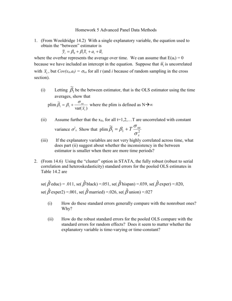
Homework 5 Advanced Panel Data Methods
1. (From Wooldridge 14.2) With a single explanatory variable, the equation used to
obtain the “between” estimator is
yi   0  1 xi  ai  ui
where the overbar represents the average over time. We can assume that E(ai) = 0
because we have included an intercept in the equation. Suppose that ui is uncorrelated
with xi , but Cov(xit,ai) = xa for all t (and i because of random sampling in the cross
section).
(i)
~
Letting 1 be the between estimator, that is the OLS estimator using the time
averages, show that
 xa
~
plim 1  1 
where the plim is defined as N
var( xi )
Assume further that the xit, for all t=1,2,…T are uncorrelated with constant
(ii)
~
variance 2x. Show that plim 1  1  T
(iii)
 xa
 x2
If the explanatory variables are not very highly correlated across time, what
does part (ii) suggest about whether the inconsistency in the between
estimator is smaller when there are more time periods?
2. (From 14.6) Using the “cluster” option in STATA, the fully robust (robust to serial
correlation and heteroskedasticity) standard errors for the pooled OLS estimates in
Table 14.2 are
se( ̂ educ) = .011, se( ̂ black) =.051, se( ̂ hispan) =.039, se( ̂ exper) =.020,
se( ̂ exper2) =.001, se( ̂ married) =.026, se( ̂ union) =.027
(i)
How do these standard errors generally compare with the nonrobust ones?
Why?
(ii)
How do the robust standard errors for the pooled OLS compare with the
standard errors for random effects? Does it seem to matter whether the
explanatory variable is time-varying or time-constant?
3. A fellow classmate has written their own code to estimate within, between, and
random effects models with balanced panels. As a check on their work, they estimate
between, within and random effects models for the one-way effects models with one
covariate.
(a) The equation that describes the fixed and random effects models is Yit=Xitβ + ui +
εit. The results are summarized below. You look at the results and tell the student
they have a programming error. What tipped you off?
Variable
Xit
Parameter Estimates and Standard Errors
Between
Fixed
0.01092
(0.00214)
0.03285
(0.00251)
Random
0.03312
(0.00267)
(b) Your classmates fixes their coding error and generates the following results for a
different problem. These are correct. What is the Hausman test statistic for the
null hypothesis that ui and Xit are uncorrelated? Can you reject or not reject the
null?
Variable
Xit
Parameter Estimates and Standard Errors
Between
Fixed
0.11012
(0.04412)
0.04813
(0.02429)
Random
0.0635
(0.02137)
4. Download the Stata dataset called panel_hw.dta. This dataset examines voter
turnout in 49 US states (Louisiana is omitted because of an unusual election in 1982)
plus the District of Columbia over 11 elections (contains data on 50 units over 11
time periods). Submit write-ups for these problems as well as the log files.
(i) Regress turnout as a percent of voting age population on the number of days
before the general election by which an individual needs to register, state per
capita income, the dummy variable for midterm elections, and the dummy
variables for West North Central, the South, and the Border states.
regress vaprate gsp midterm regdead WNCentral South Border
Which coefficients are significant? Are there any regional effects of these
regions? Use an F-test to determine this.
(ii) Part (i) assumed that pooling the data was valid. Instead, estimate this with a
fixed effects regression. Which variables are omitted from the estimation? Why?
(iii)Test for whether there is evidence of unobserved heterogeneity—that is, whether
a fixed effects model is more appropriate than the pooled model. What is your
testing hypothesis? What is your test statistic? Is pooling appropriate in light of
the results of your test?
(iv) Now estimate a random-effects model. Why do those results differ from the fixed
effects results? Is there evidence of unobserved heterogeneity? Show your
testing hypothesis, and decide on it. Are some variables omitted from the
estimation? Why or why not?
(v) Which model is more appropriate, FE or RE? What is your underlying testing
hypothesis? What implication does the null hypothesis have? Discuss the
tradeoffs between using pooled OLS, fixed-effects, and random-effects for this
model.
Some useful STATA commands for this problem:
Declare the data to be panel data before using the xtreg commands:
iis stcode declares the cross sectional units are indicated by stcode
tis year declares time periods are indicated by year.
One way to run a fixed-effects model :
xtreg vaprate midterm gsp regdead WNCentral South Border, fe
Store the estimation results with
estimates store fe
(You can replace fe in this last command with whatever name you want to use)
The bottom line of the estimation results give us an F test for pooling.
Another way to run a fixed effects model:
xi: reg vaprate midterm gsp regdead WNCentral South Border
i.stcode
Yet another way to run a fixed effects model:
areg vaprate midterm gsp regdead WNCentral South Border,
absorb(stcode)
Random effects model:
xtreg vaprate midterm gsp regdead WNCentral South Border, re
Store the estimation results with
estimates store re
(You can replace re in this last command with whatever name you want to use)
Testing commands
xttest0
xthausman
Replication Exercise
One important question in public finance is whether the structure of the welfare system
affects marriage and family formation. This assignment examines the impact of welfare
waivers (IMPDUM) on the propensity to be a never married woman (NEVERMAR).
Prior to the 1996 federal Welfare Reform Act, states could apply for waivers to
experiment with alternative systems—here related to marriage. For more information,
see Marianne Bitler, Jonah Gelbach, Hilary Hoynes, and Madeline Zovodny (2004) “The
Impact of Welfare Reform on Marriage and Divorce.”
This assignment is focused on identifying and implementing a model using variation
across states and over time in a particular policy.
Download the dataset wr-nevermar.dta. The dataset consists of a sample of black
women ages 16-54 with a high school education or less from 1989-1996. The data come
from the March CPS.
It is easy to whip through this problem. The real value here comes from spending a lot of
time thinking about what the variation in the data looks like and how that variation is
being used in the various estimates.
1. Summarize and describe the data. Graph the mean of NEVERMAR by year.
Describe the trend in this variable.
(use the egen command to create the mean of this variable by year)
2. Now graph the mean of the policy variable IMPDEM over time. How is that variable
trending over time? Discuss the trends in (1) and (2) together.
3. Collapse the data to the year level and estimate the model:
NEVERMARt = α +γIMPDUMt + et
Where is the identification coming from in this time series model? Why might this be
a biased estimate of γ? If it is biased, what do you think the key omitted variable is?
Why don’t you control for it? Does this empirical identification strategy make sense?
Don’t forget to preserve the data before you do this and restore after. Read up
on the collapse command—you want to collapse by year.
4. Now estimate a cross sectional model for 1995:
NEVERMARi,s,95 = α +γIMPDUMs,95 + εi,s,95
Where is the identification coming from in this cross sectional model? Why might
this be a biased estimate of γ? If it is biased, what do you think the key omitted
variable is? Why don’t you control for it? Does this empirical identification strategy
make sense? What if you had estimated the model using only data from 1991?
5. Now return to the full model. Estimate the simplest model
NEVERMARi,s,t = α +γIMPDUMs,t + εi,s,t
Interpret the magnitude of the coefficient on IMPDUM. (Remember when you do
that, NEVERMAR is 0/1). Is this what you expected to find? Relate your answer to
(3).
6. Reestimate the model in (5) accounting for the fact that IMPDUM varies only at the
state level, while the data is at the individual level. In STATA, use
reg yvar xvars, cluster(state)
You should cluster your standard errors for the rest of this problem.
7. Add demographic variables and economic variables to the regression (age variables,
MSADUM, URATE, EMPGRAT, RMAXPAY). Interpret the coefficient sand relate
them to what you might have predicted based on economic theory. Be careful with
units when you interpret the variables.
8. Add year fixed effects to the model (keep in the demographic and economic
variables). That is, estimate
NEVERMARi,s,t = α +γIMPDUMs,t + βX i,s,t + ηt + εi,s,t
Use the xi: reg command to do this so you can see the coefficients on the fixed
effects.
Where is the identification in THIS model coming from and how does it differ from
that in (3)? What happens to the coefficient on IMPDUM? Explain why the
coefficient changed as it did using reasoning related to omitted variable bias.
9. Add state fixed effects to the model along with the year fixed effects.
NEVERMARi,s,t = α +γIMPDUMs,t + βXi,s,t + ξs + ηt + εi,s,t
Where is the identification in THIS model coming from and how does it differ from
that in (3)? What happens to the coefficient on IMPDUM? Explain why the
coefficient changed as it did using reasoning related to omitted variable bias.
10. Add state specific time trends to the model:
NEVERMARi,s,t = α +γIMPDUMi,s,t + βX i,s,t + ΘsTime + ξs + ηt + εi,s,t
How do the results for IMPDUM change with the time trends? Explain why the
results changed.
To do this, use this command:
xi: reg yvar xvars i.year i.state*year, cluster(state)