Microsoft Word Free Math Add-In
Graph Options
Animate Command
Examples of polar graphs in two-dimensions
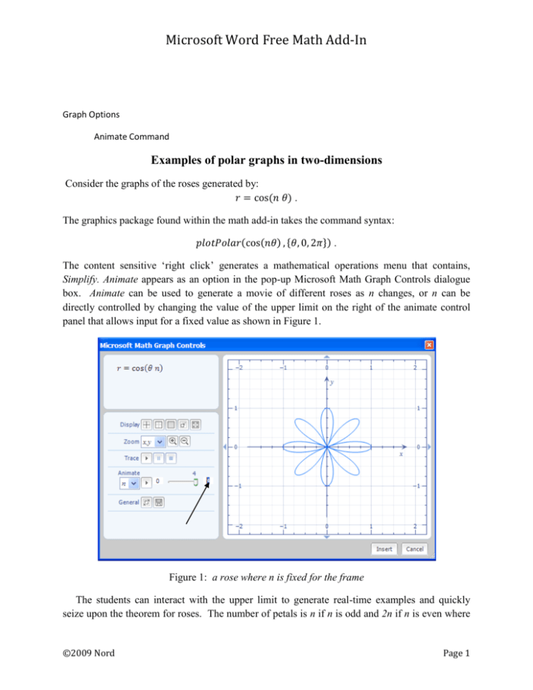
Consider the graphs of the roses generated by:
𝑟 = cos⁡(𝑛⁡𝜃) .
The graphics package found within the math add-in takes the command syntax:
𝑝𝑙𝑜𝑡𝑃𝑜𝑙𝑎𝑟(cos(𝑛𝜃) , {𝜃, 0, 2𝜋}) .
The content sensitive ‘right click’ generates a mathematical operations menu that contains,
Simplify. Animate appears as an option in the pop-up Microsoft Math Graph Controls dialogue
box. Animate can be used to generate a movie of different roses as n changes, or n can be
directly controlled by changing the value of the upper limit on the right of the animate control
panel that allows input for a fixed value as shown in Figure 1.
Figure 1: a rose where n is fixed for the frame
The students can interact with the upper limit to generate real-time examples and quickly
seize upon the theorem for roses. The number of petals is n if n is odd and 2n if n is even where
©2009 Nord
Page 1
Microsoft Word Free Math Add-In
𝑟 = sin 𝑛𝜃 or 𝑟 = cos 𝑛𝜃 [6]. The plotPolar command can be absent, and an example using
𝑟 = sin 𝑛𝜃 is given in Figure 2 using the Plot in 2D option from the pull-down screen. The input
can merely be 𝑠𝑖𝑛 𝑛𝜃 followed by a right click. The input does not require multifaceted syntax.
The animate command will appear by default with the introduction of the variable, n.
Figure 2: creating a movie with the right arrow key
Cardioids and limaçons can easily be treated with the same student interest generated by the
Animate command. Apply the Simplify option from the command, 𝑝𝑙𝑜𝑡𝑃𝑜𝑙𝑎𝑟(𝑎 +
𝑏⁡cos⁡(𝜃), {𝜃, 0, 4𝜋}) and generate a graph with default values a = b = 1. For example, b=1,
when animating on a. It is possible to introduce more than one variable for utilization of the
animate feature.
Figure 3: cardioid
©2009 Nord
Page 2
Microsoft Word Free Math Add-In
Students can discover that 𝑟 = 𝑎 + 𝑏𝑐𝑜𝑠𝜃 is the graph of a cardioid if |a| =|b| as shown in
𝑎
Figure 3. Otherwise, the graph is a limaçon that has two loops if |a| <|b|, dimpled if 1 < |𝑏| <2,
𝑎
and convex if |𝑏|≥ 2 [6].
Several real-time examples involving the ‘play’ button will lead students to conjecture and
test assumptions about the relationships between parameters a, and b, and the resulting graphs.
Serious students looking for extensions, or explorations, can be left to discover relationships
between graph types when parameters, a, b, and n, vary with the equation of 𝑟 = 𝑎 + 𝑏𝑐𝑜𝑠⁡𝑛𝜃⁡ .
The speed of computers enables students to produce many examples when exploring
mathematical problems; this supports their observation of patterns and the building and justifying
of generalizations [5].
Examples of polar graphs in three-dimensions
The free math add-in found in Microsoft Word 2007 can also generate three-dimensional polar
images, using spherical coordinates. An example of the syntax for three-dimensional polar
graphs is,
𝑝𝑙𝑜𝑡𝑃𝑜𝑙𝑎𝑟3𝐷(cos(3𝜃) sin(2𝜑) , {𝜃, 𝜋, 3𝜋}) .
The image is shown in Figure 4.
Figure 4: a three-dimensional image
The National Council of Teachers of Mathematics Curriculum Standards (1989) encourages
the use graphing utilities to investigate informally the surfaces generated by functions of two
variables. “Such investigations not only contribute to further development of important
visualization skills but also foreshadow more advanced work with functions.”
An application of the animate command to three-dimensional polar graphs could entail using
𝑝𝑙𝑜𝑡𝑃𝑜𝑙𝑎𝑟3𝐷(cos(𝑎𝜃) sin(𝑏𝜑) , {𝜃, 𝜋, 3𝜋})⁡⁡⁡⁡⁡⁡⁡or
©2009 Nord
Page 3
Microsoft Word Free Math Add-In
⁡⁡⁡⁡⁡⁡⁡⁡⁡⁡𝑝𝑙𝑜𝑡𝑃𝑜𝑙𝑎𝑟3𝐷(φcos(𝑎𝜃) , {𝜃, 0, 3𝜋}, {𝜑, 0, 𝜋}). Similarly, the option of omitting the
plotPolar3D syntax is permitted. The equation r = f(𝜃, 𝜑) can be inserted and the use of the
command Plot in 3D can be applied from the menu.
The graph generated by the math Word command, 𝑝𝑙𝑜𝑡𝑃𝑜𝑙𝑎𝑟3𝐷(𝜃𝜑, {𝜃, 0, 3𝜋}, {𝜑, 0, 𝜋}), is
the spherical coordinates three-dimensional analog to the spiral of Archimedes as seen in Figure
5 [6]. It might be very difficult to draw an example resembling a chambered nautilus on the
chalkboard of this quality. Students should use the Rotate option to revolve the surface around
the x, y, or z axis. In addition, the Zoom feature allows for further interactive investigation.
Having students use computers to manipulate pictures dynamically, encourages them to visualize
the geometry as they generate their own mental images [5].
Figure 5: image of a shell that resembles a chambered nautilus
Selected graphing commands
Table 1 contains a selection of graphing commands designed to demonstrate the versatility and
power of the software. Flexible input allows for alternative syntax. For example,
𝑝𝑙𝑜𝑡(4𝑥 2 + 12𝑥 + 2) followed with a right click and the selection of Simplify will produce the
graph of a parabola. Alternatively, the input of the expression, 4𝑥 2 + 12𝑥 + 2 , or the equation,
𝑦 = 4𝑥 2 + 12𝑥 + 2, followed with a right-click and the selection of Plot in 2D all yield the
identical graph.
©2009 Nord
Page 4
Microsoft Word Free Math Add-In
Graph Options
Graphing Commands
Table 1: other features
Command
Example
Input
plot
plot3D
plotCylDataSet3D
𝑝𝑙𝑜𝑡(4𝑥 2 + 12 ∗ 𝑥 + 2)
𝑝𝑙𝑜𝑡3𝐷(2𝑥 + 𝑦 3 )
Input function, f(x).
Input where, z=f(x, y).
Data point is {𝑟, 𝜃, 𝑧}.
plotCylParamLine3D
𝜋
𝑝𝑙𝑜𝑡𝐶𝑦𝑙𝐷𝑎𝑡𝑎𝑆𝑒𝑡3𝐷({{2, 1, 5}, {5, , 1}})
3
2 ),
𝑝𝑙𝑜𝑡𝐶𝑦𝑙𝑃𝑎𝑟𝑎𝑚𝐿𝑖𝑛𝑒3𝐷(2𝑡, 𝑠𝑖𝑛(𝑡 2𝑡)
plotIneq
𝑝𝑙𝑜𝑡𝐶𝑦𝑙𝑅3𝐷(𝑟 2 + 𝑠𝑖𝑛(2𝜃))
𝑝𝑙𝑜𝑡𝐷𝑎𝑡𝑎𝑆𝑒𝑡({{2, −7}, {−1, −12}})
𝑝𝑙𝑜𝑡𝐷𝑎𝑡𝑎𝑆𝑒𝑡3𝐷({{20, 0, 19}, {−6, 12, 22}})⁡
𝑝𝑙𝑜𝑡𝐸𝑞(𝑥 2 + 𝑦 2 = 4)
𝑥2
𝑝𝑙𝑜𝑡𝐸𝑞3𝐷( + 𝑦 2 + 𝑧 2 = 1)
9
𝑝𝑙𝑜𝑡𝐼𝑛𝑒𝑞(2𝑥 ≤ 3 + 3𝑦)
plotParam
𝑝𝑙𝑜𝑡𝑃𝑎𝑟𝑎𝑚(𝑠𝑖𝑛 𝑡, 3𝑡 − 5)
plotParam3D
𝑝𝑙𝑜𝑡𝑃𝑎𝑟𝑎𝑚3𝐷(𝑡 + 𝑠 2 , 𝑡 + 3𝑠, 𝑡 − 𝑠 2 )
plotParamLine3D
𝑝𝑙𝑜𝑡𝑃𝑎𝑟𝑎𝑚𝐿𝑖𝑛𝑒3𝐷(𝑐𝑜𝑠(3𝑡), 𝑡 + 5, 𝑡 3 )
plotPolarDataSet
𝜋
𝜋
𝑝𝑙𝑜𝑡𝑃𝑜𝑙𝑎𝑟𝐷𝑎𝑡𝑎𝑆𝑒𝑡({{14, } , {8, − }})
3
3
𝜋
𝜋 𝜋
𝑝𝑙𝑜𝑡𝑃𝑜𝑙𝑎𝑟𝐷𝑎𝑡𝑎𝑆𝑒𝑡3𝐷({{3, , 𝜋} , {29, , }})
6
2 8
plotCylR3D
plotDataSet
plotDataSet3D
plotEq
plotEq3D
plotPolarDataSet3D
Insert 𝑟 = 𝑓(𝑡), 𝑧 =
𝑔(𝑡), 𝜃 = ℎ(𝑡).
Input z=f(r, 𝜃).
Input point, {x, y}.
Input point, {x, y, z}.
Input f(x, y) = c.
Input f(x, y, z)=c.
Input inequality in x
and y.
Input (f(t), g(t)) where
x=f(t) and y=g(t).
Input (f(t, s), g(t, s),
h(t, s)) where x=f(t, s)
and
y=g(t, s) and z=h(t, s).
Input ( f(t), g(t), h(t))
where x=f(t) and
y=g(t)and z=h(t).
Input point {𝑟, 𝜃}.
Input a point, {𝑟, 𝜃, 𝜑}.
To execute these commands using the drop-down menu, apply Calculate or Simplify.
©2009 Nord
Page 5
Microsoft Word Free Math Add-In
Example 1: Use the plotParam3D command.
Input:
𝑝𝑙𝑜𝑡𝑃𝑎𝑟𝑎𝑚3𝐷(cosh 𝑠 cos 𝑡, sin 𝑠 cos 𝑡, sin 𝑡)
Output:
Example 2: Use the plotparamline3d command.
Input:
𝑝𝑙𝑜𝑡𝑝𝑎𝑟𝑎𝑚3𝑑(cos 𝑡⁡, sin 𝑡, cos 𝑡 sin 𝑠𝑡)
Output:
©2009 Nord
Page 6
Microsoft Word Free Math Add-In
Example 3: Sketch the intersection of two cylinders, x2+y2=1 and z2+y2=1.
Input:
𝑝𝑙𝑜𝑡𝑝𝑎𝑟𝑎𝑚𝑙𝑖𝑛𝑒3𝑑(cos 𝑡, sin 𝑡, cos 𝑡)
Output:
©2009 Nord
Page 7
Microsoft Word Free Math Add-In
Using the show3d command, plotting the two cylinders on the same axes is possible using one input
line.
Input:
𝑠ℎ𝑜𝑤3𝑑(𝑃𝑙𝑜𝑡𝑒𝑞3𝑑(𝑥 2 + 𝑦 2 = 1), 𝑝𝑙𝑜𝑡𝑒𝑞3𝑑(𝑧 2 + 𝑦 2 = 1))
Output:
Example 4: Use the plot3d command.
Input:
3
𝑝𝑙𝑜𝑡3𝑑(√𝑥 3 + 𝑦 3 )
Output:
©2009 Nord
Page 8
Microsoft Word Free Math Add-In
©2009 Nord
Page 9
Microsoft Word Free Math Add-In
References
1. International Society for Technology in Education (ISTE) (2009). ISTE’s U.S. Public
Policy Principles and Federal & State Objectives. Washington, D.C.:
http://www.iste.org/Content/NavigationMenu/Advocacy/Policy/109.09-US-PublicPolicy-Principles.pdf
2. Microsoft Corporation, Word 2007 Math Add-In:
http://www.microsoft.com/downloads/details.aspx?familyid=030FAE9C-704F-48CA971D-56241AEFC764&displaylang=en.
3. National Council of Teachers of Mathematics (NCTM) (1989). Curriculum and
Evaluation Standards for School Mathematics. NCTM, Reston, Virginia.
4. National Council of Teachers of Mathematics (NCTM) (2000). Principles and
Standards for School Mathematics. NCTM, Reston, Virginia.
5. Oldknow, A. (ed.) (2005). ICT and Mathematics: a guide to learning and teaching
mathematics 11-19. The Mathematical Association, Leicester.
6. Repka, J. (1994). Calculus with Analytic Geometry. Wm. C. Brown, Dubuque, Iowa.
7. Riddle, D. (1984). Calculus and Analytic Geometry. fourth edition, Wadsworth,
Belmont, California.
8. Shepard, M., (1997). A rose is a rose is a rose…. The College Mathematics Journal, 28
No 1, 55-56.
9. Stewart, J. (2003). Calculus. fifth edition, Thomson Learning, Belmont, California,
2003.
10. Thomas, G. and Finney, R. Calculus and Analytic Geometry, 9th edition, AddisonWesley, Reading, Massachusetts, 1996.
©2009 Nord
Page 10
Microsoft Word Free Math Add-In
Graph Options
Show and Show3D commands
Use the Show command when working in two dimensions. Use the Show3D command when working in
three dimensions. The show and show3d commands are used to input more than one curve/surface
with one input line. The multiple curves/surfaces will appear graphed together. Separate each
curve/surface with a comma.
Example 1: Give an example using the show3d command and the plot3d command.
Input:
𝑠ℎ𝑜𝑤3𝐷(𝑝𝑙𝑜𝑡3𝑑(𝑦 2 − 𝑥 2 ), 𝑝𝑙𝑜𝑡3𝑑(𝑥 2 + 𝑦 2 ))
Output:
©2009 Nord
Page 11
Microsoft Word Free Math Add-In
Change the
scale.
Change the
scale here
for specific
values.
Change the scale if you want by using the last two buttons in the Display row. A new window yields:
After right-clicking on the input line, select Simplify from the menu to bring up the graph.
Example 2: Give an example using the show3d command and the plotparamline3d command.
Input:
𝑠ℎ𝑜𝑤3𝑑(𝑝𝑙𝑜𝑡𝐸𝑞3𝐷(𝑥 2 + 𝑦 2 + 𝑧 2 = 1), 𝑝𝑙𝑜𝑡𝑝𝑎𝑟𝑎𝑚𝑙𝑖𝑛𝑒3𝑑(cos 𝑡, sin 𝑡, cos 𝑡))
©2009 Nord
Page 12
Microsoft Word Free Math Add-In
Output:
Example 3: Give an example using the show command, the plot command, and the deriv command.
Input:
𝑠ℎ𝑜𝑤(𝑃𝑙𝑜𝑡(𝑥 3 , {𝑥, −5,5}), 𝑃𝑙𝑜𝑡(𝑑𝑒𝑟𝑖𝑣(𝑥 3 , 𝑥), {𝑥, −5,5})
Output:
©2009 Nord
Page 13
Microsoft Word Free Math Add-In
Example 4: Give an example using the show command, the plot command, and derivn command. (The
derivn command is used when considering a nth derivative.)
Input:
𝑠ℎ𝑜𝑤(𝑃𝑙𝑜𝑡(𝑥 3 , {𝑥, −5,5}), 𝑃𝑙𝑜𝑡(𝑑𝑒𝑟𝑖𝑣(𝑥 3 , 𝑥), {𝑥, −5,5}), 𝑃𝑙𝑜𝑡(𝑑𝑒𝑟𝑖𝑣𝑛(𝑥 3 , 𝑥, 3), {𝑥, −5,5})
Output:
Example 5: Give an example using the show3d command, the plot3d command, and the animation
feature.
Input:
𝑠ℎ𝑜𝑤3𝐷(𝑃𝑙𝑜𝑡3𝐷(1 − 𝑎𝑥 3 ), 𝑃𝑙𝑜𝑡3𝐷(3𝑥 2 + 4𝑦))
©2009 Nord
Page 14
Microsoft Word Free Math Add-In
Output:
©2009 Nord
Page 15
Microsoft Word Free Math Add-In
Graph Options
Restricting Domain
Restrict the domain using this format: {variable, minimum value,maximum value}.
Example 1: Give an example restricting the domain and use the plot3d command.
Input:
𝑝𝑙𝑜𝑡3𝐷(𝑥 2 + 𝑦 2 , {𝑥, 0,4}, {𝑦, 0,6})
Output:
Example 2: Give an example restricting the domain and use the plot3d command and the show3d
command.
Input:
𝑠ℎ𝑜𝑤3𝑑(𝑝𝑙𝑜𝑡3𝐷(𝑥 2 + 𝑦 2 , {𝑥, 0,4}, {𝑦, 0,6}), 𝑝𝑙𝑜𝑡3𝐷(𝑥 − 𝑦, {𝑥, 4,10}, {𝑦, 6,12}))
Output:
©2009 Nord
Page 16
Microsoft Word Free Math Add-In
Example 3: Give an example restricting the domain where a variable is defined for negative real
numbers and use the plot3d command and the show3d command.
Input:
𝑠ℎ𝑜𝑤3𝑑(𝑝𝑙𝑜𝑡3𝐷(𝑥 3 − 𝑦 3 , {𝑥, 0,8}, {𝑦, −6,6}), 𝑝𝑙𝑜𝑡3𝐷(𝑥 4 − 𝑦 3 , {𝑥, −5,0}, {𝑦, −5,5}))
Output:
©2009 Nord
Page 17
Microsoft Word Free Math Add-In
Example 4: Give a graphing example involving a radical. In addition, restrict the domain, use the plot3d
command, and the show3d command.
Input:
5
𝑠ℎ𝑜𝑤3𝑑(𝑝𝑙𝑜𝑡3𝐷(𝑥 3 − 𝑦^3, {𝑥, 0,8}, {𝑦, −6,6}), 𝑝𝑙𝑜𝑡3𝐷 (√𝑥 4 − 𝑦^15, {𝑥, −5,0}, {𝑦, −5,5}))
Output:
©2009 Nord
Page 18
Microsoft Word Free Math Add-In
©2009 Nord
Page 19
Microsoft Word Free Math Add-In
Graph Options
Labeling Axes
Use the command alias followed by a variable to label a specific axis. The example, {aliasy,profit}, labels
the y-axis as profit.
Example 1: Give an example using the show command and plot command. Label the y-axis, ‘Profit’.
Input:
𝑠ℎ𝑜𝑤(𝑃𝑙𝑜𝑡(𝑥 2 , {𝑥, 0,4}), 𝑃𝑙𝑜𝑡(2𝑥, {𝑥, 4,10}), {𝐴𝑙𝑖𝑎𝑠𝑦,Profit})
Output:
Example 2: Give an example labeling the x-axis as Time and the y-axis as Profit.
Input:
𝑠ℎ𝑜𝑤(𝑃𝑙𝑜𝑡(2𝑥, {𝑥, 4,10}), {𝑎𝑙𝑖𝑎𝑠𝑦,Profit}, {𝑎𝑙𝑖𝑎𝑠𝑥, 𝑇𝑖𝑚𝑒})
Output:
©2009 Nord
Page 20
Microsoft Word Free Math Add-In
Use the Zoom feature to zoom in and out. The labeling of the axes are visible after zooming out. Notice
the variable x is defined in the equation as Time and the variable y is defined in the equation as Profit.
Zoom in.
Zoom out.
©2009 Nord
Page 21
Microsoft Word Free Math Add-In
Graphic Options
Color Options
When more than one graph is created, the Microsoft Word Math Add-In sets each graph a
different color by default. It is possible to specify a particular color for a curve/surface. Specify
the color using the format, {color,”RGB number”}. Double quotes are needed with the RGB
number.
The RGB number represents three two digit numbers in base 16 (with no spaces or commas). A
base 16 (hexadecimal) possible digits are 0, 1, 2, 3, 4, 5, 6, 7, 8, 9, a, b, c, d, e, and f. The
smallest two digit number in base 16 is 00 and the largest is ff. Three two digit numbers (base
16) represent the RGB (red, green, and blue) intensity respectively. The three two digit numbers
ff2200 will specify orange. Using this notation of the RGB number being ff2200, the intensity of
red is increased, the intensity of green is small, and the intensity of blue is the smallest.
In addition, the shade of a color can be controlled. If two digits are added in front of the RGB
number, the shading of the color can range from being transparent (disappear) to bold. The two
digit hexadecimal number 00 will display an invisible graph. The two digit hexadecimal number
ff will display the color in bold form. If no shade of the color is specified, the color will be in
bold form.
Example 1: Give an example of a graph that will have the color orange.
Input:
𝑝𝑙𝑜𝑡(cos 2𝑥, {𝑐𝑜𝑙𝑜𝑟, "ff2200"})⁡
Output:
©2009 Nord
Page 22
Microsoft Word Free Math Add-In
Example 2: Give an example of a graph that will have the color light orange.
Input:
𝑝𝑙𝑜𝑡(cos 2𝑥, {𝑐𝑜𝑙𝑜𝑟, "44ff2200"})
Output:
©2009 Nord
Page 23
Microsoft Word Free Math Add-In
Example 3: Give an example using the show3d command and specify a color for one of the curves.
Input:
𝑠ℎ𝑜𝑤3𝑑(𝑝𝑙𝑜𝑡𝐸𝑞3𝐷(𝑥 2 + 𝑦 2 + 𝑧 2
= 1), 𝑝𝑙𝑜𝑡𝑝𝑎𝑟𝑎𝑚𝑙𝑖𝑛𝑒3𝑑(cos 𝑡
/ cosh 𝑎𝑡 , sin 𝑡/ cosh 𝑎𝑡 , sinh 𝑎𝑡⁡/ cosh 𝑎𝑡, {𝑡, −4⁡𝜋, 4⁡𝜋}, {𝑐𝑜𝑙𝑜𝑟, "ff0000"})
Output:
©2009 Nord
Page 24
Microsoft Word Free Math Add-In
In the example, the color of the loxodrome was established to be displayed in red by setting the RGB
number to be ff0000 (Nord and Miller, 1996). The intensity of red was increased and the intensity of
green and blue were set to the lowest possible numbers. The unit sphere was displayed in a mesh
(skeleton) form by using the third button in the Display row.
©2009 Nord
Page 25
Microsoft Word Free Math Add-In
Create a
skeleton
(mesh) of the
curve.
The Microsoft Math Graph Controls box can be omitted by selecting the first button in the General row.
The second button will save the image. Below is the output after selecting the first button.
©2009 Nord
Page 26
Microsoft Word Free Math Add-In
Graphs that are not displayed in the mesh (skeleton) mode may also be saved and inserted into
documents, also. An example is shown below.
©2009 Nord
Page 27
Microsoft Word Free Math Add-In
©2009 Nord
Page 28
Microsoft Word Free Math Add-In
Graph Options
Line Styles
Equations and inequalities are plotted as solid lines (or curves) by default. The following are line
styles:





Solid
Dot
Dash
Dashdot
Dashdotdot
The format to indicate a line style is {linestyle,”type”}. Use the recognized command, linestyle,
and the double quotation marks.
Example 1: Give an example using the line style “dot” in a graphing problem.
Input:
𝑝𝑙𝑜𝑡(cos 2𝑥 , {𝑙𝑖𝑛𝑒𝑠𝑡𝑦𝑙𝑒, "dot"})
Output:
©2009 Nord
Page 29
Microsoft Word Free Math Add-In
Example 2: Give an example using the line style “dashdotdot” in a graphing problem.
Input:
𝑝𝑙𝑜𝑡(cos 2𝑥 , {𝑙𝑖𝑛𝑒𝑠𝑡𝑦𝑙𝑒, "dashdotdot"})
Output:
©2009 Nord
Page 30
Microsoft Word Free Math Add-In
©2009 Nord
Page 31
Microsoft Word Free Math Add-In
References:
Nord, J. and Miller, E. "Mercator's Rhumb Lines," The College Mathematics Journal, Mathematical
Association of America, Vol. 27, No. 5, November 1996,pages 384-387.
Thomas, G. and Finney, R. Calculus and Analytic Geometry, 9th edition, Addison-Wesley, Reading,
Massachusetts, 1996.
Zill, Dennis G. and Cullen, Michael R. Advanced Engineering Mathematics, 3rd edition, Jones and Bartlett
Publishers, Massachusetts, 2006.
http://mathworld.wolfram.com/SphericalSpiral.html
©2009 Nord
Page 32
Microsoft Word Free Math Add-In
Graph Options
Embed a Graphical Image
Embed a Graphical Image
Consider the 3-D surface, 𝑥 2 − 4𝑦 2 = 𝑧.
Right click below and select Plot in 3D.
𝑥 2 − 4𝑦 2
To embed a cropped graphical image for our example, follow these steps.
1. Select Print Screen from the top row of your computer keyboard.
2. To copy this image select Ctrl followed with c. This will copy the image.
3. Close the window of the graphing image. There is an “X” on the top right of the image.
4. Paste the desired image at a specific location within the Word document. Select Ctrl followed
with a p. This will paste the image.
Below is our example:
©2009 Nord
Page 33
Microsoft Word Free Math Add-In
5. Double-click somewhere within the graphing image.
6. Locate Picture Tools that now appears above Format on the top-most ribbon.
7. Select Crop. It now appears on the top right-hand side of the ribbon. It was must be selected
before any cropping of the image can occur. The corners will appear in black.
8. Place the cursor in the bottom right corner of the original image. Each corner will appear as
shown below. The example below is a bottom left corner.
Point and click and drag the piece off you wish. The bottom of our original image has been
cropped.
©2009 Nord
Page 34
Microsoft Word Free Math Add-In
Crop from
this corner
in the next
step.
9. Repeat the steps to crop the top part of our image. Double click on the image. Select Crop.
Now, place the cursor at the top left corner. Point and click and drag the piece off you wish here.
The resulting desired image is below:
©2009 Nord
Page 35
Microsoft Word Free Math Add-In
©2009 Nord
Page 36