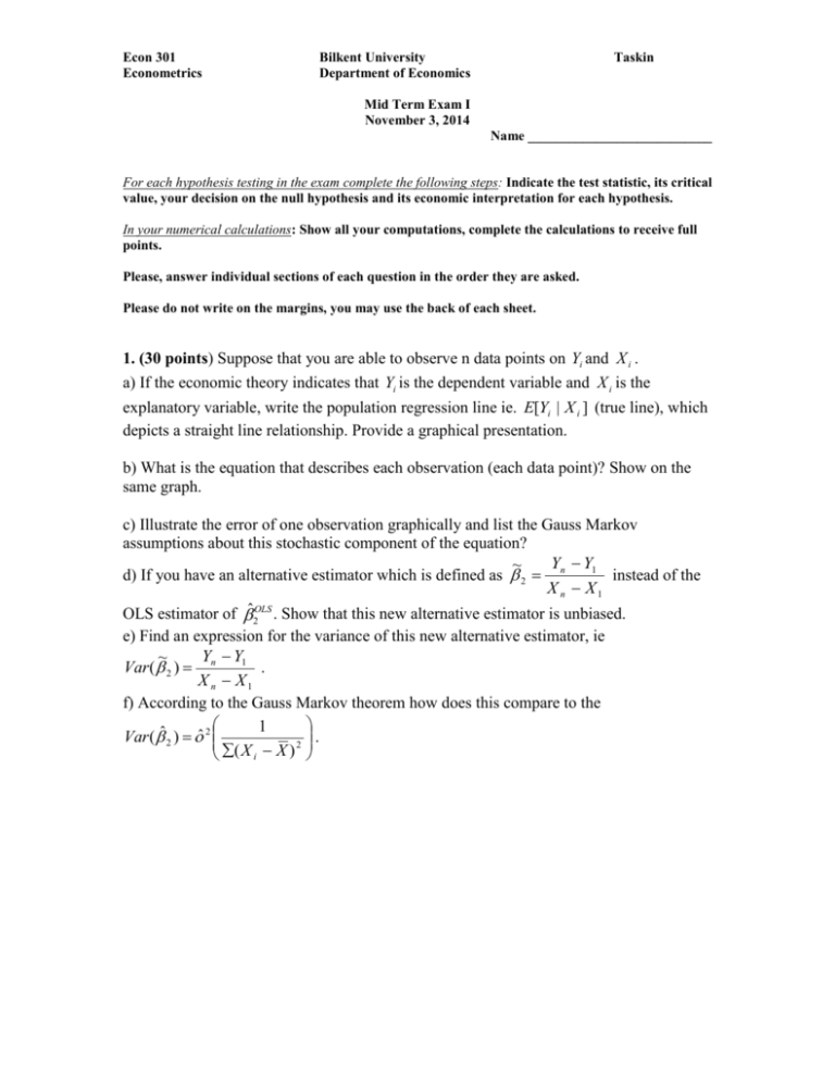
Econ 301
Econometrics
Bilkent University
Department of Economics
Taskin
Mid Term Exam I
November 3, 2014
Name ___________________________
For each hypothesis testing in the exam complete the following steps: Indicate the test statistic, its critical
value, your decision on the null hypothesis and its economic interpretation for each hypothesis.
In your numerical calculations: Show all your computations, complete the calculations to receive full
points.
Please, answer individual sections of each question in the order they are asked.
Please do not write on the margins, you may use the back of each sheet.
1. (30 points) Suppose that you are able to observe n data points on Yi and X i .
a) If the economic theory indicates that Yi is the dependent variable and X i is the
explanatory variable, write the population regression line ie. E[Yi | X i ] (true line), which
depicts a straight line relationship. Provide a graphical presentation.
b) What is the equation that describes each observation (each data point)? Show on the
same graph.
c) Illustrate the error of one observation graphically and list the Gauss Markov
assumptions about this stochastic component of the equation?
Y  Y1
~
d) If you have an alternative estimator which is defined as  2  n
instead of the
X n  X1
OLS estimator of b̂2OLS . Show that this new alternative estimator is unbiased.
e) Find an expression for the variance of this new alternative estimator, ie
Y  Y1
~
.
Var (  2 )  n
X n  X1
f) According to the Gauss Markov theorem how does this compare to the


1
.
Var (ˆ 2 )  ˆ 2 
2 

(
X

X
)
i


Name ___________________________
2. (20 points) (Derivation of the OLS estimator) In the following model,
Yi  1   2 X 2i   3 X 3i  ui
a) Write the fitted equation and define the residual.
b) Write the expression for the sum of squared residual.
c) Minimize the SSR with respect to 1 ,  2 and b3.
d) Prove that derivation of the OLS estimators b̂1, b̂2 and b̂3. uses the two following
normal equations:
 X 2i uˆi  0 and  X 3i uˆi  0 . Is the condition  uˆi  0 satisfied in this model?
2
Name ___________________________
3. (20 points) The following food consumption function Yi  1   2 X i  ui is estimated
for the sample of 40 families and the results of the estimation is :
Yˆi  40.76  0.1283 X i .
a) Compute the fitted value of food consumption for the income level of X 0  750
dollars.
b) Write the formula for Vaˆr ( ˆ 2 ) and compute the Vaˆr ( ˆ 2 ) .
c) Compute a 95% confidence interval for the slope coefficient.
d) Test the hypothesis of the significance of the slope coefficient.
[ ˆ  37.8 , Y  130.31 X  698.00 , ( X i  X ) 2  28200,
(Yi  Y ) 2  2038 ]
3
Name ___________________________
4. (30 points) The Economics department of a major university keeps track of its majors’
starting salaries. The data on the salaries (SALARY) in UD dollars and the Grade Point
Average (GPA) of 50 graduates are used to estimate the following regression equation:
Salary i    GPAi  ui where all the standard conditions of the model are
assumed.
Eviews estimation results are presented below:
============================================================
Dependent Variable: SALARY
Method: Least Squares
Date: 10/18/05 Time: 11:03
Sample: 1 50
Included observations: 50
============================================================
Variable
Coefficient
Std. Error
t-Statistic
Prob.
============================================================
C
27199.78
1956.161
13.90467
0.0000
GPA
1101.126
653.9115
1.683907
0.0987
============================================================
R-squared
0.055779
Mean dependent var 30430.92
Adjusted R-squared
0.036107
S.D. dependent var
2739.002
S.E. of regression
2689.098
Akaike info criteri
18.67098
Sum squared resid 347 000 000
Schwarz criterion
18.74746
Log likelihood
-464.7744
F-statistic
2.835542
Durbin-Watson stat
0.632309
Prob(F-statistic)
0.098693
a. Write the estimated (fitted) equation.
b. Give the economic interpretation of the intercept and slope coefficients of this
model.
c. Compute the Unexplained (residual) Sum of Squares, Explained Sum of Squares
and Total Sum of Squares, and interpret R2.
d. Test the following hypothesis 0.05 significance level.
H o :   0,
HA :   0
According to the results of this hypothesis is GPA a relevant variable in
explaining the starting salary of Economics graduates.
e. Test the following hypothesis 0.05 significance level.
H o :   1000,
H A :   1000
f. If the alternative model Salary i    ui ' is estimated and the Sum of Squared
Residual is equal to SSR=367 498 000, test the validity of this restriction. State
what is the null hypothesis associated with the restriction and perform a formal
test.
[Indicate the test statistic, its critical value, your decision on the null hypothesis and
its economic interpretation for each hypothesis]
4
Name ___________________________
5
Name ___________________________
6
Name ___________________________
FORMULA SHEET
ˆ 2 =
nå X iYi - å X i åYi
nå X - (å X i )
2
i
ˆ1 = Y - b2 X =
=
2
å( X - X )(Y -Y )
å( X - X )
i
i
2
i
å X åY - å X å X Y
nå X - (å X )
2
i
i
2
i
i
where i = 1….n
i i
2
i
where i = 1….n

 X 2i
2
ˆ


ˆ
Var ( 1 )   
2 
n

(
X

X
)
i




1

Var ( ˆ2 )  ˆ 2 
2 
 ( X i  X ) 


X

Cov( ˆ1 ˆ 2 )  ˆ 2 
2 

(
X

X
)
i


sˆ 2 =
t stat 
R2 
å ûi2
n-K
ˆ j   j
seˆ( ˆ j )
SSE
SSR
 1
SST
SST
R 2  1
SSE is sum of squared explained, SSR is sum of squared residuals
SSR /( n  K )
TSS /( n  1)
Var ( x  y )  Var ( x)  Var ( y )  2Cov( xy)
F  stat 
SSRR  SSRU /( J )
SSRU /( n  K )
  e 2  2k
AIC  ln  i  
 n  n
7
Name ___________________________
8
Name ___________________________
9