MODEL Statement
<label:> MODEL dependents=<regressors> < / options > ;
After the keyword MODEL, the dependent (response) variables are specified, followed by an
equal sign and the regressor variables. Variables specified in the MODEL statement must be
numeric variables in the data set being analyzed. For example, if you want to specify a
quadratic term for variable X1 in the model, you cannot use X1*X1 in the MODEL statement
but must create a new variable (for example, X1SQUARE=X1*X1) in a DATA step and use
this new variable in the MODEL statement. The label in the MODEL statement is optional.
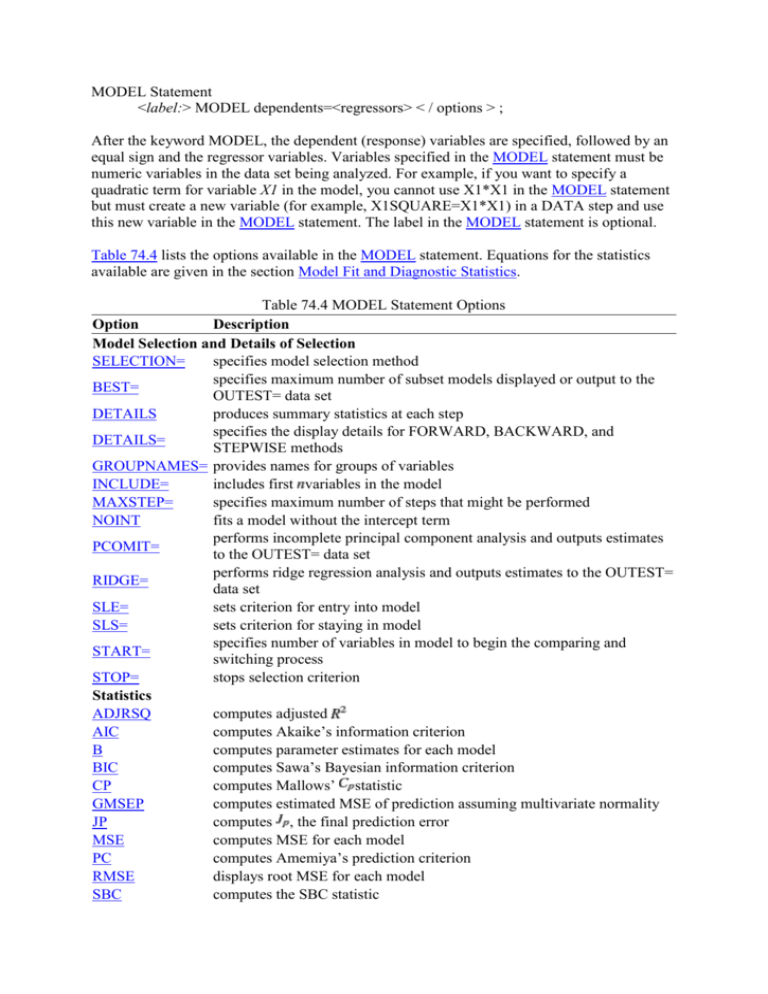
Table 74.4 lists the options available in the MODEL statement. Equations for the statistics
available are given in the section Model Fit and Diagnostic Statistics.
Table 74.4 MODEL Statement Options
Option
Description
Model Selection and Details of Selection
SELECTION=
specifies model selection method
specifies maximum number of subset models displayed or output to the
BEST=
OUTEST= data set
DETAILS
produces summary statistics at each step
specifies the display details for FORWARD, BACKWARD, and
DETAILS=
STEPWISE methods
GROUPNAMES= provides names for groups of variables
INCLUDE=
includes first variables in the model
MAXSTEP=
specifies maximum number of steps that might be performed
NOINT
fits a model without the intercept term
performs incomplete principal component analysis and outputs estimates
PCOMIT=
to the OUTEST= data set
performs ridge regression analysis and outputs estimates to the OUTEST=
RIDGE=
data set
SLE=
sets criterion for entry into model
SLS=
sets criterion for staying in model
specifies number of variables in model to begin the comparing and
START=
switching process
STOP=
stops selection criterion
Statistics
ADJRSQ
computes adjusted
AIC
computes Akaike’s information criterion
B
computes parameter estimates for each model
BIC
computes Sawa’s Bayesian information criterion
CP
computes Mallows’ statistic
GMSEP
computes estimated MSE of prediction assuming multivariate normality
JP
computes , the final prediction error
MSE
computes MSE for each model
PC
computes Amemiya’s prediction criterion
RMSE
displays root MSE for each model
SBC
computes the SBC statistic
SP
computes statistic for each model
SSE
computes error sum of squares for each model
Data Set Options
outputs the number of regressors, the error degrees of freedom, and the
EDF
model to the OUTEST= data set
outputs standard errors of the parameter estimates to the OUTEST= data
OUTSEB
set
outputs standardized parameter estimates to the OUTEST= data set. Use
OUTSTB
only with the RIDGE= or PCOMIT= option.
outputs the variance inflation factors to the OUTEST= data set. Use only
OUTVIF
with the RIDGE= or PCOMIT= option.
PRESS
outputs the PRESS statistic to the OUTEST= data set
RSQUARE
has same effect as the EDF option
Regression Calculations
I
displays inverse of sums of squares and crossproducts
XPX
displays sums-of-squares and crossproducts matrix
Details on Estimates
displays heteroscedasticity- consistent covariance matrix of estimates and
ACOV
heteroscedasticity-consistent standard errors
specifies method for computing the asymptotic heteroscedasticityACOVMETHOD=
consistent covariance matrix
COLLIN
produces collinearity analysis
COLLINOINT
produces collinearity analysis with intercept adjusted out
CORRB
displays correlation matrix of estimates
COVB
displays covariance matrix of estimates
HCC
displays heteroscedasticity-consistent standard errors
specifies method for computing the asymptotic heteroscedasticityHCCMETHOD=
consistent covariance matrix
LACKFIT
performs lack-of-fit test
displays squared semipartial correlation coefficients computed using Type
PARTIALR2
I sums of squares
displays squared partial correlation coefficients computed using Type I
PCORR1
sums of squares
displays squared partial correlation coefficients computed using Type II
PCORR2
sums of squares
displays squared semipartial correlation coefficients computed using Type
SCORR1
I sums of squares
displays squared semipartial correlation coefficients computed using Type
SCORR2
II sums of squares
SEQB
displays a sequence of parameter estimates during selection process
SPEC
tests that first and second moments of model are correctly specified
SS1
displays the sequential sums of squares
SS2
displays the partial sums of squares
STB
displays standardized parameter estimates
TOL
displays tolerance values for parameter estimates
WHITE
displays heteroscedasticity-consistent standard errors
VIF
computes variance-inflation factors
Predicted and Residual Values
CLB
computes
% confidence limits for the parameter estimates
CLI
computes
% confidence limits for an individual predicted value
computes
% confidence limits for the expected value of the
CLM
dependent variable
DW
computes a Durbin-Watson statistic
DWPROB
computes a Durbin-Watson statistic and -value
INFLUENCE
computes influence statistics
P
computes predicted values
PARTIAL
displays partial regression plots for each regressor
PARTIALDATA displays partial regression data
R
produces analysis of residuals
Display Options and Other Options
requests the following options:
ACOV, CLB, CLI, CLM, CORRB, COVB, HCC, I, P,
ALL
PCORR1, PCORR2, R, SCORR1, SCORR2, SEQB, SPEC,
SS1, SS2, STB, TOL, VIF, XPX
ALPHA=
sets significance value for confidence and prediction intervals and tests
NOPRINT
suppresses display of results
specifies the true standard deviation of error term for computing CP and
SIGMA=
BIC
SINGULAR=
sets criterion for checking for singularity
You can specify the following options in the MODEL statement after a slash (/).
ACOV
displays the estimated asymptotic covariance matrix of the estimates under the
hypothesis of heteroscedasticity and heteroscedasticity-consistent standard errors of
parameter estimates. See the HCCMETHOD= option and the HCC option and the
section Testing for Heteroscedasticity for more information.
ACOVMETHOD=0,1,2, or 3
See the HCCMETHOD= option.
ADJRSQ
computes adjusted for degrees of freedom for each model selected (Darlington
1968; Judge et al. 1980).
AIC
outputs Akaike’s information criterion for each model selected (Akaike 1969; Judge et
al. 1980) to the OUTEST= data set. If SELECTION=ADJRSQ,
SELECTION=RSQUARE, or SELECTION=CP is specified, then the AIC statistic is
also added to the SubsetSelSummary table.
ALL
requests all these options: ACOV, CLB, CLI, CLM, CORRB, COVB, HCC, I, P,
PCORR1, PCORR2, R, SCORR1, SCORR2, SEQB, SPEC, SS1, SS2, STB, TOL,
VIF, and XPX.
ALPHA=number
sets the significance level used for the construction of confidence intervals for the
current MODEL statement. The value must be between 0 and 1; the default value of
0.05 results in 95% intervals. This option affects the MODEL options CLB, CLI, and
CLM; the OUTPUT statement keywords LCL, LCLM, UCL, and UCLM; the PLOT
statement keywords LCL., LCLM., UCL., and UCLM.; and the PLOT statement
options CONF and PRED. If you specify this option in the MODEL statement, it takes
precedence over the ALPHA= option in the PROC REG statement.
B
is used with the RSQUARE, ADJRSQ, and CP model-selection methods to compute
estimated regression coefficients for each model selected.
BEST=n
is used with the RSQUARE, ADJRSQ, and CP model-selection methods. If
SELECTION=CP or SELECTION=ADJRSQ is specified, the BEST= option specifies
the maximum number of subset models to be displayed or output to the OUTEST=
data set. For SELECTION=RSQUARE, the BEST= option requests the maximum
number of subset models for each size.
If the BEST= option is used without the B option (displaying estimated regression
coefficients), the variables in each MODEL are listed in order of inclusion instead of
the order in which they appear in the MODEL statement.
If the BEST= option is omitted and the number of regressors is less than 11, all
possible subsets are evaluated. If the BEST= option is omitted and the number of
regressors is greater than 10, the number of subsets selected is, at most, equal to the
number of regressors. A small value of the BEST= option greatly reduces the CPU
time required for large problems.
BIC
outputs Sawa’s Bayesian information criterion for each model selected (Sawa 1978;
Judge et al. 1980) to the OUTEST= data set. If SELECTION=ADJRSQ,
SELECTION=RSQUARE, or SELECTION=CP is specified, then the BIC statistic is
also added to the SubsetSelSummary table.
CLB
requests the
% upper and lower confidence limits for the parameter
estimates. By default, the 95% limits are computed; the ALPHA= option in the PROC
REG or MODEL statement can be used to change the level. If any of the MODEL
statement options ACOV, HCC, or WHITE are in effect, then the CLB option also
produces heteroscedasticity-consistent
% upper and lower confidence limits
for the parameter estimates.
CLI
requests the
% upper and lower confidence limits for an individual predicted
value. By default, the 95% limits are computed; the ALPHA= option in the PROC
REG or MODEL statement can be used to change the level. The confidence limits
reflect variation in the error, as well as variation in the parameter estimates. See the
section Predicted and Residual Values and Chapter 4, Introduction to Regression
Procedures, for more information.
CLM
displays the
% upper and lower confidence limits for the expected value of
the dependent variable (mean) for each observation. By default, the 95% limits are
computed; the ALPHA= in the PROC REG or MODEL statement can be used to
change the level. This is not a prediction interval (see the CLI option) because it
takes into account only the variation in the parameter estimates, not the variation in the
error term. See the section Predicted and Residual Values and Chapter 4, Introduction
to Regression Procedures, for more information.
COLLIN
requests a detailed analysis of collinearity among the regressors. This includes
eigenvalues, condition indices, and decomposition of the variances of the estimates
with respect to each eigenvalue. See the section Collinearity Diagnostics.
COLLINOINT
requests the same analysis as the COLLIN option with the intercept variable adjusted
out rather than included in the diagnostics. See the section Collinearity Diagnostics.
CORRB
displays the correlation matrix of the estimates. This is the
unit diagonals.
matrix scaled to
COVB
displays the estimated covariance matrix of the estimates. This matrix is
where is the estimated mean squared error.
CP
,
outputs Mallows’ statistic for each model selected (Mallows 1973; Hocking 1976)
to the OUTEST= data set. See the section Criteria Used in Model-Selection Methods
for a discussion of the use of . If SELECTION=ADJRSQ,
SELECTION=RSQUARE, or SELECTION=CP is specified, then the statistic is
also added to the SubsetSelSummary table.
DETAILS
DETAILS=name
specifies the level of detail produced when the BACKWARD, FORWARD, or
STEPWISE method is used, where name can be ALL, STEPS, or SUMMARY. The
DETAILS or DETAILS=ALL option produces entry and removal statistics for each
variable in the model building process, ANOVA and parameter estimates at each step,
and a selection summary table. The option DETAILS=STEPS provides the step
information and summary table. The option DETAILS=SUMMARY produces only
the summary table. The default if the DETAILS option is omitted is
DETAILS=STEPS.
DW
calculates a Durbin-Watson statistic to test whether or not the errors have first-order
autocorrelation. (This test is appropriate only for time series data.) Note that your data
should be sorted by the date/time ID variable before you use this option. The sample
autocorrelation of the residuals is also produced. See the section Autocorrelation in
Time Series Data.
DWPROB
calculates a Durbin-Watson statistic and a -value to test whether or not the errors
have first-order autocorrelation. Note that it is not necessary to specify the DW option
if the DWPROB option is specified. (This test is appropriate only for time series data.)
Note that your data should be sorted by the date/time ID variable before you use this
option. The sample autocorrelation of the residuals is also produced. See the section
Autocorrelation in Time Series Data.
EDF
outputs the number of regressors in the model excluding and including the intercept,
the error degrees of freedom, and the model to the OUTEST= data set.
GMSEP
outputs the estimated mean square error of prediction assuming that both independent
and dependent variables are multivariate normal (Stein 1960; Darlington 1968) to the
OUTEST= data set. (Note that Hocking’s formula (1976, eq. 4.20) contains a misprint:
"
" should read "
.") If SELECTION=ADJRSQ, SELECTION=RSQUARE, or
SELECTION=CP is specified, then the GMSEP statistic is also added to the
SubsetSelSummary table.
GROUPNAMES=’name1’ ’name2’ ...
provides names for variable groups. This option is available only in the
BACKWARD, FORWARD, and STEPWISE methods. The group name can be up to
32 characters. Subsets of independent variables listed in the MODEL statement can be
designated as variable groups. This is done by enclosing the appropriate variables in
braces. Variables in the same group are entered into or removed from the regression
model at the same time. However, if the tolerance of any variable (see the TOL
option) in a group is less than the setting of the SINGULAR= option, then the variable
is not entered into the model with the rest of its group. If the GROUPNAMES= option
is not used, then the names GROUP1, GROUP2, ..., GROUPn are assigned to groups
encountered in the MODEL statement. Variables not enclosed by braces are used as
groups of a single variable.
For example:
model y={x1 x2} x3 / selection=stepwise
groupnames='x1 x2' 'x3';
Another example:
model y={ht wgt age} bodyfat / selection=forward
groupnames='htwgtage' 'bodyfat';
HCC
requests heteroscedasticity-consistent standard errors of the parameter estimates. You
can use the HCCMETHOD= option to specify the method used to compute the
heteroscedasticity-consistent covariance matrix.
HCCMETHOD=0,1,2, or 3
specifies the method used to obtain a heteroscedasticity-consistent covariance matrix
for use with the ACOV, HCC, or WHITE option in the MODEL statement and for
heteroscedasticity-consistent tests with the TEST statement. The default is
HCCMETHOD=0. See the section Testing for Heteroscedasticity for details.
I
displays the
matrix. The inverse of the crossproducts matrix is bordered by the
parameter estimates and SSE matrices.
INCLUDE=n
forces the first n independent variables listed in the MODEL statement to be included
in all models. The selection methods are performed on the other variables in the
MODEL statement. The INCLUDE= option is not available with
SELECTION=NONE.
INFLUENCE
requests a detailed analysis of the influence of each observation on the estimates and
the predicted values. See the section Influence Statistics for details.
JP
outputs , the estimated mean square error of prediction for each model selected
assuming that the values of the regressors are fixed and that the model is correct to the
OUTEST= data set. The statistic is also called the final prediction error (FPE) by
Akaike (Nicholson 1948; Lord 1950; Mallows 1967; Darlington 1968; Rothman 1968;
Akaike 1969; Hocking 1976; Judge et al. 1980). If SELECTION=ADJRSQ,
SELECTION=RSQUARE, or SELECTION=CP is specified, then the statistic is
also added to the SubsetSelSummary table.
LACKFIT
performs a lack-of-fit test. See the section Testing for Lack of Fit for more
information. Refer to Draper and Smith (1981) for a discussion of lack-of-fit tests.
MSE
computes the mean square error for each model selected (Darlington 1968).
MAXSTEP=n
specifies the maximum number of steps that are done when
SELECTION=FORWARD, SELECTION=BACKWARD, or
SELECTION=STEPWISE is used. The default value is the number of independent
variables in the model for the FORWARD and BACKWARD methods and three times
this number for the stepwise method.
NOINT
suppresses the intercept term that is otherwise included in the model.
NOPRINT
suppresses the normal display of regression results. Note that this option temporarily
disables the Output Delivery System (ODS); see Chapter 20, Using the Output
Delivery System, for more information.
OUTSEB
outputs the standard errors of the parameter estimates to the OUTEST= data set. The
value SEB for the variable _TYPE_ identifies the standard errors. If the RIDGE= or
PCOMIT= option is specified, additional observations are included and identified by
the values RIDGESEB and IPCSEB, respectively, for the variable _TYPE_. The
standard errors for ridge regression estimates and incomplete principal components
(IPC) estimates are limited in their usefulness because these estimates are biased. This
option is available for all model-selection methods except RSQUARE, ADJRSQ, and
CP.
OUTSTB
outputs the standardized parameter estimates as well as the usual estimates to the
OUTEST= data set when the RIDGE= or PCOMIT= option is specified. The values
RIDGESTB and IPCSTB for the variable _TYPE_ identify ridge regression estimates
and IPC estimates, respectively.
OUTVIF
outputs the variance inflation factors (VIF) to the OUTEST= data set when the
RIDGE= or PCOMIT= option is specified. The factors are the diagonal elements of
the inverse of the correlation matrix of regressors as adjusted by ridge regression or
IPC analysis. These observations are identified in the output data set by the values
RIDGEVIF and IPCVIF for the variable _TYPE_.
P
calculates predicted values from the input data and the estimated model. The display
includes the observation number, the ID variable (if one is specified), the actual and
predicted values, and the residual. If the CLI, CLM, or R option is specified, the P
option is unnecessary. See the section Predicted and Residual Values for more
information.
PARTIAL
requests partial regression leverage plots for each regressor. You can use the
PARTIALDATA option to obtain a tabular display of the partial regression leverage
data. If ODS Graphics is in effect (see the section ODS Graphics), then these partial
plots are produced in panels with up to six plots per panel. See the section Influence
Statistics for more information.
PARTIALDATA
requests partial regression leverage data for each regressor. You can request partial
regression leverage plots of these data with the PARTIAL option. See the section
Influence Statistics for more information.
PARTIALR2 <( < TESTS> <SEQTESTS> ) >
See the SCORR1 option.
PC
outputs Amemiya’s prediction criterion for each model selected (Amemiya 1976;
Judge et al. 1980) to the OUTEST= data set. If SELECTION=ADJRSQ,
SELECTION=RSQUARE, or SELECTION=CP is specified, then the PC statistic is
also added to the SubsetSelSummary table.
PCOMIT=list
requests an IPC analysis for each value m in the list. The procedure computes
parameter estimates by using all but the last m principal components. Each value of m
produces a set of IPC estimates, which is output to the OUTEST= data set. The values
of m are saved by the variable _PCOMIT_, and the value of the variable _TYPE_ is
set to IPC to identify the estimates. Only nonnegative integers can be specified with
the PCOMIT= option.
If you specify the PCOMIT= option, RESTRICT statements are ignored. The
PCOMIT= option is ignored if you use the SELECTION= option in the MODEL
statement.
PCORR1
displays the squared partial correlation coefficients computed using Type I sum of
squares (SS). This is calculated as SS/(SS+SSE), where SSE is the error sum of
squares.
PCORR2
displays the squared partial correlation coefficients computed using Type II sums of
squares. These are calculated the same way as with the PCORR1 option, except that
Type II SS are used instead of Type I SS.
PRESS
outputs the PRESS statistic to the OUTEST= data set. The values of this statistic are
saved in the variable _PRESS_. This option is available for all model-selection
methods except RSQUARE, ADJRSQ, and CP.
R
requests an analysis of the residuals. The results include everything requested by the P
option plus the standard errors of the mean predicted and residual values, the
studentized residual, and Cook’s statistic to measure the influence of each
observation on the parameter estimates. See the section Predicted and Residual Values
for more information.
RIDGE=list
requests a ridge regression analysis and specifies the values of the ridge constant k
(see the section Computations for Ridge Regression and IPC Analysis). Each value of
k produces a set of ridge regression estimates that are placed in the OUTEST= data
set. The values of k are saved by the variable _RIDGE_, and the value of the variable
_TYPE_ is set to RIDGE to identify the estimates.
Only nonnegative numbers can be specified with the RIDGE= option. Example 74.5
illustrates this option.
If you specify the RIDGE= option, RESTRICT statements are ignored. The RIDGE=
option is ignored if you use the SELECTION= option in the MODEL statement.
RMSE
displays the root mean square error for each model selected.
RSQUARE
has the same effect as the EDF option.
SBC
outputs the SBC statistic for each model selected (Schwarz 1978; Judge et al. 1980) to
the OUTEST= data set. If SELECTION=ADJRSQ, SELECTION=RSQUARE, or
SELECTION=CP is specified, then the SBC statistic is also added to the
SubsetSelSummary table.
SCORR1 <( < TESTS> <SEQTESTS> ) >
displays the squared semipartial correlation coefficients computed using Type I sums
of squares. This is calculated as SS/SST, where SST is the corrected total SS. If the
NOINT option is used, the uncorrected total SS is used in the denominator. The
optional arguments TESTS and SEQTESTS request are sequentially added to a model.
The -test values are computed as the Type I sum of squares for the variable in
question divided by a mean square error. If you specify the TESTS option, the
denominator MSE is the residual mean square for the full model specified in the
MODEL statement. If you specify the SEQTESTS option, the denominator MSE is the
residual mean square for the model containing all the independent variables that have
been added to the model up to and including the variable in question. The TESTS and
SEQTESTS options are not supported if you specify model selection methods or the
RIDGE or PCOMIT options. Note that the PARTIALR2 option is a synonym for the
SCORR1 option.
SCORR2 <( TESTS )>
displays the squared semipartial correlation coefficients computed using Type II sums
of squares. These are calculated the same way as with the SCORR1 option, except that
Type II SS are used instead of Type I SS. The optional TEST argument requests tests
and -values as variables are sequentially added to a model. The -test values are
computed as the Type II sum of squares for the variable in question divided by the
residual mean square for the full model specified in the MODEL statement. The
TESTS option is not supported if you specify model selection methods or the RIDGE
or PCOMIT options.
SELECTION=name
specifies the method used to select the model, where name can be FORWARD (or F),
BACKWARD (or B), STEPWISE, MAXR, MINR, RSQUARE, ADJRSQ, CP, or
NONE (use the full model). The default method is NONE. See the section ModelSelection Methods for a description of each method.
SEQB
produces a sequence of parameter estimates as each variable is entered into the model.
This is displayed as a matrix where each row is a set of parameter estimates.
SIGMA=n
specifies the true standard deviation of the error term to be used in computing the CP
and BIC statistics. If the SIGMA= option is not specified, an estimate from the full
model is used. This option is available in the RSQUARE, ADJRSQ, and CP modelselection methods only.
SINGULAR=n
tunes the mechanism used to check for singularities. If you specify this option in the
MODEL statement, it takes precedence over the SINGULAR= option in the PROC
REG statement. The default value is machine dependent but is approximately 1E 7 on
most machines. This option is rarely needed. Singularity checking is described in the
section Computational Methods.
SLENTRY=value
SLE=value
specifies the significance level for entry into the model used in the FORWARD and
STEPWISE methods. The defaults are 0.50 for FORWARD and 0.15 for STEPWISE.
SLSTAY=value
SLS=value
specifies the significance level for staying in the model for the BACKWARD and
STEPWISE methods. The defaults are 0.10 for BACKWARD and 0.15 for
STEPWISE.
SP
outputs the statistic for each model selected (Hocking 1976) to the OUTEST= data
set. If SELECTION=ADJRSQ, SELECTION=RSQUARE, or SELECTION=CP is
specified, then the SP statistic is also added to the SubsetSelSummary table.
SPEC
performs a test that the first and second moments of the model are correctly specified.
See the section Testing for Heteroscedasticity for more information.
SS1
displays the sequential sums of squares (Type I SS) along with the parameter estimates
for each term in the model. See Chapter 15, The Four Types of Estimable Functions,
for more information about the different types of sums of squares.
SS2
displays the partial sums of squares (Type II SS) along with the parameter estimates
for each term in the model. See the SS1 option also.
SSE
computes the error sum of squares for each model selected.
START=s
is used to begin the comparing-and-switching process in the MAXR, MINR, and
STEPWISE methods for a model containing the first independent variables in the
MODEL statement, where is the START value. For these methods, the default is
START=0.
For the RSQUARE, ADJRSQ, and CP methods, START= specifies the smallest
number of regressors to be reported in a subset model. For these methods, the default
is START=1.
The START= option cannot be used with model-selection methods other than the six
described here.
STB
produces standardized regression coefficients. A standardized regression coefficient is
computed by dividing a parameter estimate by the ratio of the sample standard
deviation of the dependent variable to the sample standard deviation of the regressor.
STOP=s
causes PROC REG to stop when it has found the "best" -variable model, where is
the STOP value. For the RSQUARE, ADJRSQ, and CP methods, STOP= specifies
the largest number of regressors to be reported in a subset model. For the MAXR and
MINR methods, STOP= specifies the largest number of regressors to be included in
the model.
The default setting for the STOP= option is the number of variables in the MODEL
statement. This option can be used only with the MAXR, MINR, RSQUARE,
ADJRSQ, and CP methods.
TOL
produces tolerance values for the estimates. Tolerance for a variable is defined as
, where is obtained from the regression of the variable on all other regressors
in the model. See the section Collinearity Diagnostics for more details.
VIF
produces variance inflation factors with the parameter estimates. Variance inflation is
the reciprocal of tolerance. See the section Collinearity Diagnostics for more detail.
WHITE
See the HCC option.
XPX
displays the
crossproducts matrix for the model. The crossproducts matrix is
bordered by the
and
matrices.