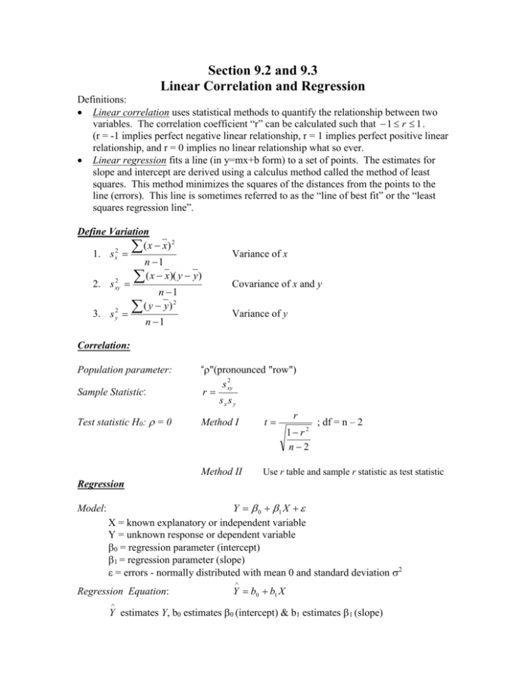
Section 9.2 and 9.3
Linear Correlation and Regression
Definitions:
 Linear correlation uses statistical methods to quantify the relationship between two
variables. The correlation coefficient “r” can be calculated such that  1  r  1 .
(r = -1 implies perfect negative linear relationship, r = 1 implies perfect positive linear
relationship, and r = 0 implies no linear relationship what so ever.
 Linear regression fits a line (in y=mx+b form) to a set of points. The estimates for
slope and intercept are derived using a calculus method called the method of least
squares. This method minimizes the squares of the distances from the points to the
line (errors). This line is sometimes referred to as the “line of best fit” or the “least
squares regression line”.
Define Variation
 ( x  x) 2
1. s x2 
n 1
 ( x  x)( y  y)
2. s xy2 
n 1
( y  y) 2

2
3. s y 
n 1
Variance of x
Covariance of x and y
Variance of y
Correlation:
Population parameter:
Sample Statistic:
Test statistic H0: = 0
“"(pronounced "row")
s xy2
r
sx s y
r
t
Method I
; df = n – 2
1 r2
n2
Method II
Use r table and sample r statistic as test statistic
Regression
Model:
Y   0  1 X  
X = known explanatory or independent variable
Y = unknown response or dependent variable
0 = regression parameter (intercept)
1 = regression parameter (slope)
 = errors - normally distributed with mean 0 and standard deviation 2

Regression Equation:

Y  b0  b1 X
Y estimates Y, b0 estimates 0 (intercept) & b1 estimates 1 (slope)
s xy2
Parameter estimates:
b1 
Relationship between r and b1:
b1 
Residuals (e):
e  ( y  y)
b0  y  b1 x
;
s x2
rs y
r
so
sx
b1 s x
; derived using algebra
sy

Standard error of Residuals:
se 
Standard error of b1:
sb1 
e
n2

2
n2
se
s x (n  1)
Test statistic H0: 1 = 0
Confidence interval for 1:

 ( y  y)
2
t
b1   1
; df = n – 2
sb1
b1  t sb1  1  b1  t sb1
2

Standard error of y (mean value):
2
2
1 ( x p  x)

n  ( x  x) 2
s   se
y
Confidence interval for y:


y  t  s    y  y  t s 
2

s
Confidence interval for Ynew:
y  t s

2
y
2
1 ( x p  x)
1 
n  ( x  x) 2
 se
Standard error of y (new individual value):
( y y)
y



2 ( y y)
 Ynew  y  t s

2 ( y y)
Correlation and Regression Steps
1. Plot a Scatter Diagram
2. Calculate the correlation coefficient “r”
3. Test the significance of “r” ; H0:  = 0
4. Determine least squares regression line
a. Verify the relationship between “r” and “b1”
b. Plot regression line on scatter plot – start at ( x, y ) and use slope
to find 2nd point, then draw line.
5. Calculate
se
and
sb1 (must first find  e 2 )
6. Determine if x is useful in predicting y ; H0: 1 = 0
7. Construct a confidence interval for 1
8. Prediction
a. Find prediction value
b. Calculate prediction interval (mean and new individual value)
Most of these quantities can be found in the excel regression output or from
calculator functions which you are incouraged to use, however you are still
responsible for understanding concepts and relationships.